Визуализация данных в R

.title[
# Визуализация данных в R
]
.subtitle[
## base r, ggplot2, plotly etc..
]
.author[
### Полина и Лена
]
.date[
### 2023/03/20 (updated: 2023-03-26)
]

---

# baser r plots
---
### Важность визуализации
.pull-left[
<img src="img/ex.jfif">
]
.pull-right[
<img src="img/dino.jfif">
]
---
### Какие можно вспомнить виды графиков?

- Диаграмма рассеяния (scatterplot)
 
--

- Гистограмма (histogram)
 
--

- Барплот (barplot)
 
--

**Чем барплот отличается от гистограммы?**

Гистограммы для непрерывных величин, а барплоты для категориальных.

- Боксплот (boxplot)

- Скрипичная диаграмма (violin plot)

- Pie chart (не рекомендуется)

- Диаграмма Венна

- Heatmap, density plot, upset, flowchart и много чего еще…
 
---
# mtcars
Мы будем работать с датасетом `mtcars` (Motor Trend Car Road Tests)
--
 Чтобы посмотреть описание датасета вобьем в консоль

```r
?mtcars
```
--
A data frame with 32 observations on 11 (numeric) variables.
 [, 1]	mpg	Miles/(US) gallon
 [, 2]	cyl	Number of cylinders
 [, 3]	disp	Displacement (cu.in.)
 [, 4]	hp	Gross horsepower
 [, 5]	drat	Rear axle ratio
 [, 6]	wt	Weight (1000 lbs)
 [, 7]	qsec	1/4 mile time
 [, 8]	vs	Engine (0 = V-shaped, 1 = straight)
 [, 9]	am	Transmission (0 = automatic, 1 = manual)
 [,10]	gear	Number of forward gears
 [,11]	carb	Number of carburetors
---
# mtcars
<div class="datatables html-widget html-fill-item-overflow-hidden html-fill-item" id="htmlwidget-4d67a8704d8dab2425e0" style="width:100%;height:auto;"></div>
<script type="application/json" data-for="htmlwidget-4d67a8704d8dab2425e0">{"x":{"filter":"none","vertical":false,"fillContainer":false,"data":[["Mazda RX4","Mazda RX4 Wag","Datsun 710","Hornet 4 Drive","Hornet Sportabout","Valiant","Duster 360","Merc 240D","Merc 230","Merc 280","Merc 280C","Merc 450SE","Merc 450SL","Merc 450SLC","Cadillac Fleetwood","Lincoln Continental","Chrysler Imperial","Fiat 128","Honda Civic","Toyota Corolla","Toyota Corona","Dodge Challenger","AMC Javelin","Camaro Z28","Pontiac Firebird","Fiat X1-9","Porsche 914-2","Lotus Europa","Ford Pantera L","Ferrari Dino","Maserati Bora","Volvo 142E"],[21,21,22.8,21.4,18.7,18.1,14.3,24.4,22.8,19.2,17.8,16.4,17.3,15.2,10.4,10.4,14.7,32.4,30.4,33.9,21.5,15.5,15.2,13.3,19.2,27.3,26,30.4,15.8,19.7,15,21.4],[6,6,4,6,8,6,8,4,4,6,6,8,8,8,8,8,8,4,4,4,4,8,8,8,8,4,4,4,8,6,8,4],[160,160,108,258,360,225,360,146.7,140.8,167.6,167.6,275.8,275.8,275.8,472,460,440,78.7,75.7,71.1,120.1,318,304,350,400,79,120.3,95.1,351,145,301,121],[110,110,93,110,175,105,245,62,95,123,123,180,180,180,205,215,230,66,52,65,97,150,150,245,175,66,91,113,264,175,335,109],[3.9,3.9,3.85,3.08,3.15,2.76,3.21,3.69,3.92,3.92,3.92,3.07,3.07,3.07,2.93,3,3.23,4.08,4.93,4.22,3.7,2.76,3.15,3.73,3.08,4.08,4.43,3.77,4.22,3.62,3.54,4.11],[2.62,2.875,2.32,3.215,3.44,3.46,3.57,3.19,3.15,3.44,3.44,4.07,3.73,3.78,5.25,5.424,5.345,2.2,1.615,1.835,2.465,3.52,3.435,3.84,3.845,1.935,2.14,1.513,3.17,2.77,3.57,2.78],[16.46,17.02,18.61,19.44,17.02,20.22,15.84,20,22.9,18.3,18.9,17.4,17.6,18,17.98,17.82,17.42,19.47,18.52,19.9,20.01,16.87,17.3,15.41,17.05,18.9,16.7,16.9,14.5,15.5,14.6,18.6],[0,0,1,1,0,1,0,1,1,1,1,0,0,0,0,0,0,1,1,1,1,0,0,0,0,1,0,1,0,0,0,1],[1,1,1,0,0,0,0,0,0,0,0,0,0,0,0,0,0,1,1,1,0,0,0,0,0,1,1,1,1,1,1,1],[4,4,4,3,3,3,3,4,4,4,4,3,3,3,3,3,3,4,4,4,3,3,3,3,3,4,5,5,5,5,5,4],[4,4,1,1,2,1,4,2,2,4,4,3,3,3,4,4,4,1,2,1,1,2,2,4,2,1,2,2,4,6,8,2]],"container":"<table class=\"display\">\n <thead>\n <tr>\n <th> <\/th>\n <th>mpg<\/th>\n <th>cyl<\/th>\n <th>disp<\/th>\n <th>hp<\/th>\n <th>drat<\/th>\n <th>wt<\/th>\n <th>qsec<\/th>\n <th>vs<\/th>\n <th>am<\/th>\n <th>gear<\/th>\n <th>carb<\/th>\n <\/tr>\n <\/thead>\n<\/table>","options":{"pageLength":6,"columnDefs":[{"className":"dt-right","targets":[1,2,3,4,5,6,7,8,9,10,11]},{"orderable":false,"targets":0}],"order":[],"autoWidth":false,"orderClasses":false,"lengthMenu":[6,10,25,50,100]}},"evals":[],"jsHooks":[]}</script>
---
# mtcars
.left-column[
Чтобы посмотреть описательные статистики датасета наберем в консоли:

```r
summary(mtcars)
```
 
 
 
 
 
 
 
 
 
]
.right-column[

```
## mpg cyl disp hp 
## Min. :10.40 Min. :4.000 Min. : 71.1 Min. : 52.0 
## 1st Qu.:15.43 1st Qu.:4.000 1st Qu.:120.8 1st Qu.: 96.5 
## Median :19.20 Median :6.000 Median :196.3 Median :123.0 
## Mean :20.09 Mean :6.188 Mean :230.7 Mean :146.7 
## 3rd Qu.:22.80 3rd Qu.:8.000 3rd Qu.:326.0 3rd Qu.:180.0 
## Max. :33.90 Max. :8.000 Max. :472.0 Max. :335.0 
## drat wt qsec vs 
## Min. :2.760 Min. :1.513 Min. :14.50 Min. :0.0000 
## 1st Qu.:3.080 1st Qu.:2.581 1st Qu.:16.89 1st Qu.:0.0000 
## Median :3.695 Median :3.325 Median :17.71 Median :0.0000 
## Mean :3.597 Mean :3.217 Mean :17.85 Mean :0.4375 
## 3rd Qu.:3.920 3rd Qu.:3.610 3rd Qu.:18.90 3rd Qu.:1.0000 
## Max. :4.930 Max. :5.424 Max. :22.90 Max. :1.0000 
## am gear carb 
## Min. :0.0000 Min. :3.000 Min. :1.000 
## 1st Qu.:0.0000 1st Qu.:3.000 1st Qu.:2.000 
## Median :0.0000 Median :4.000 Median :2.000 
## Mean :0.4062 Mean :3.688 Mean :2.812 
## 3rd Qu.:1.0000 3rd Qu.:4.000 3rd Qu.:4.000 
## Max. :1.0000 Max. :5.000 Max. :8.000
```
]
---
# Диаграмма рассеяния (scatterplot)
.pull-left[
```r
plot(mtcars$mpg)
```
 На диаграмме рассеяния каждому наблюдению соответствует точка, координаты которой равны значениям двух каких-то параметров этого наблюдения.
 
 mpg - расход топлива
 **index** - порядок значений колонки mpg в таблице

]
.pull-right[
![](rvisualisation_files/figure-html/unnamed-chunk-5-1.png)
]
---
# Scatterplots
.pull-left[
```r
plot(x = mtcars$disp, y = mtcars$mpg)
```
равнозначные обозначения
```r
plot(mtcars$disp ~ mtcars$mpg)
```
 
 mpg - расход топлива (Miles/(US) gallon)
 нарисуем зависимость mpg от displacement 
]
.pull-right[
![](rvisualisation_files/figure-html/unnamed-chunk-6-1.png)

]
---
# Scatterplots
.pull-left[
```r
plot(mtcars$wt,
* type="b")
```
аргумент **type =.** 
 type = "p", default
 just lines (type = "l") 
 both points and lines connected (type = "b")
 both points and lines with the lines running through the points (type = "o")
 empty points joined by lines (type = "c")
]
.pull-right[
![](rvisualisation_files/figure-html/unnamed-chunk-7-1.png)
]
---

# Histograms
.pull-left[
 Позволяет быстро посмотреть на распределение своих данных

```r
hist(mtcars$cyl)
```
 По оси **х** - частота или количество машин с конкретным количеством цилиндров (**cyl**)

наглядное представление функции плотности вероятности некоторой случайной величины, построенное по выборке
]
.pull-right[

![](rvisualisation_files/figure-html/unnamed-chunk-9-1.png)
]
---
# Histograms
.pull-left[
```r
hist(mtcars$wt, 
*main = "Title", ylab="y", xlab="x",
*col="coral", border="blue")
```
]
.pull-right[
![](rvisualisation_files/figure-html/unnamed-chunk-10-1.png)
]
---
# Histograms
.pull-left[
```r
hist(mtcars$wt, 
 main = "Title", ylab="y", xlab="x",
* col = rainbow(25), 
 border="blue")
```
rainbow() автоматически применяет градиент от красного к зеленому

```r
 rainbow(5)
```

```
## [1] "#FF0000" "#CCFF00" "#00FF66" "#0066FF" "#CC00FF"
```
]
.pull-right[
![](rvisualisation_files/figure-html/unnamed-chunk-12-1.png)
]
---
# Histograms
.pull-left[
```r
hist(mtcars$wt, 
 main = "Title", ylab="y", xlab="x",
* col = terrain.colors(12), 
 border="blue")
```
Можно поэкспериментировать с числом, которое подается функции **terrain.colors()**
]
.pull-right[
![](rvisualisation_files/figure-html/unnamed-chunk-13-1.png)
]
---

# Оффтопик
.pull-left[
base r pallets

```r
head(hcl.pals())
```

```
## [1] "Pastel 1" "Dark 2" "Dark 3" "Set 2" "Set 3" "Warm"
```
пример использования
```r
hist(mtcars$wt, 
 main = "Title", ylab="y", xlab="x",
* col = hcl.colors(20,"Pastel 1"), 
 border="blue")
```
]
.pull-right[
![](rvisualisation_files/figure-html/unnamed-chunk-15-1.png)

rainbow(n, s = 1, v = 1, start = 0, end = max(1, n - 1)/n,
 alpha, rev = FALSE)
 heat.colors(n, alpha, rev = FALSE)
 terrain.colors(n, alpha, rev = FALSE)
 topo.colors(n, alpha, rev = FALSE)
 cm.colors(n, alpha, rev = FALSE)
 [Rcolor.pdf](http://www.stat.columbia.edu/~tzheng/files/Rcolor.pdf)
]
---
# Histograms
.pull-left[
```r
hist(mtcars$wt, 
 main = "Title", ylab="y", xlab="x",
 col = terrain.colors(12), 
 border="blue",
* freq = FALSE)
```
По умолчанию по оси **у** отложена частота (frequency)
 Если выставить freq = FALSE значение на оси **у** изменится на пллотность (density)
 Данные разбиты на **bins**, каждый бин - интервал данных.
]
.pull-right[

![](rvisualisation_files/figure-html/unnamed-chunk-16-1.png)
]
---
# Histograms
.pull-left[
```r
hist(mtcars$wt, 
 main = "Title", ylab="y", xlab="x",
 col = terrain.colors(12), 
 border="blue",
 freq = FALSE)
*lines(density(mtcars$wt))
```
]
.pull-right[
![](rvisualisation_files/figure-html/unnamed-chunk-17-1.png)
]
---

# Boxplot
.pull-left[
```r
boxplot(mtcars$mpg, ylab = "y")
```
график, использующийся в описательной статистике, компактно изображающий одномерное распределение вероятностей.
 
 Такой вид диаграммы в удобной форме показывает **медиану** (или, если нужно, среднее), нижний и верхний **квартили**, **минимальное** и **максимальное** значение выборки и **выбросы**.

]
.pull-right[

![](rvisualisation_files/figure-html/unnamed-chunk-18-1.png)
]
---
# Boxplot
.pull-left[
```r
boxplot(mtcars$mpg ~ mtcars$cyl, 
* main = "Title",
* col="lightblue")
```
Дополнительная кастомизация
]
.pull-right[
![](rvisualisation_files/figure-html/unnamed-chunk-19-1.png)
]
---
.pull-left[
### Другие типы плотов в base r
```r
par(mfrow=c(3, 1))
### stripchart()
stripchart(mtcars$mpg,
 main = "Mpg",
 method="jitter",
 col = "orange",
 pch=10)
### barplot()
barplot(mtcars$mpg[1:6], 
main = "Первые 6 наблюдений расхода топлива", 
 ylab = "Miles/(US) gallon",
 names.arg = row.names(mtcars)[1:6],
 col = terrain.colors(10)
)
### q-q plot 
qqnorm(mtcars$mpg, pch = 1, frame = FALSE)
qqline(mtcars$mpg, col = "steelblue", lwd = 2)
```
Для дальнейшей кастомизации: [CheatSheet](https://r-graph-gallery.com/6-graph-parameters-reminder.html)
]
.pull-right[
![](rvisualisation_files/figure-html/unnamed-chunk-20-1.png)
]
---

# ggplot2!!
---
.pull-left[
### Grammar of graphics
 
 
 Подход к построению графиков в `ggplot2` принципиально отличается от обычных пакетов визуализации (matplotlib, seaborn в питоне). 
 Фишка `ggplot2` состоит в применении языка грамматики графики - набора правил для построения графиков. 
 Такой подход дает огромную гибкость и возможность создания и кастомизации практически любого графика. Пакет опирается на книгу The Grammar of Graphics (Leland Wilkinson).
]
.pull-right[
<img src="img/gg.jfif">
]
---
class: fullscreen, top, center
background-image: url("img/ggp.jfif")

.right[https://twitter.com/tanya_shapiro/status/1576935152575340544]
---
# ggplot2
 [ggplot2 tutorial](https://ggplot2.tidyverse.org)
 Установка библиотеки:

```r
install.packages("ggplot2")
```
`ggplot2` входит в core `tidyverse`, так что если вы уже установили `tidyverse` отдельно устанавливать `ggplot2` не надо
---
# wc3_units
<div class="datatables html-widget html-fill-item-overflow-hidden html-fill-item" id="htmlwidget-a9eb5a91fec307a8a057" style="width:100%;height:auto;"></div>
<script type="application/json" data-for="htmlwidget-a9eb5a91fec307a8a057">{"x":{"filter":"none","vertical":false,"data":[["1","2","3","4","5","6","7","8","9","10","11","12","13","14","15","16","17","18","19","20","21","22","23","24","25","26","27","28","29","30","31","32","33","34","35","36","37","38","39","40","41","42","43","44","45","46","47","48","49","50","51","52","53","54","55","56","57","58","59","60","61","62","63","64","65","66","67","68","69","70","71"],["Peasant","Militia","Footman","Rifleman","Knight","Priest","Sorceress","Spell Breaker","Flying Machine","Mortar Team","Siege Engine","Gryphon Rider","Dragonhawk Rider","Water Elemental 1","Water Elemental 2","Water Elemental 3","Phoenix","Peon","Grunt","T. Headhunter","T. Berserker","Demolisher","Raider","Tauren","Shaman","Witch Doctor","Spirit Walker","Kodo Beast","Wind Rider","Troll Batrider","Spirit Wolf","Dire Wolf","Shadow Wolf","Serpent Ward","Wisp","Archer","Huntress","Glaive Thrower","Dryad","DoC Druid Form","DoC Bear Form","Mountain Giant","Mountain Giant 2","Hippogryph","DoT Druid Form","DoT Crow Form","Faerie Dragon","Hippogryph Rider","Chimaera","Chimaera 2","Treant","Avatar of Vengeance","Spirit of Vengeance","Acolyte","Ghoul","Crypt Fiend","Gargoyle","Abomination","Meat Wagon","Necromancer","Banshee","Frost Wyrm","Shade","Skeleton Warrior","Skeletal Mage","Infernal","Carrion Beetle 1","Carrion Beetle 2","Carrion Beetle 3","Obsidian Statue","Destroyer"],["Human","Human","Human","Human","Human","Human","Human","Human","Human","Human","Human","Human","Human","Human","Human","Human","Human","Orc","Orc","Orc","Orc","Orc","Orc","Orc","Orc","Orc","Orc","Orc","Orc","Orc","Orc","Orc","Orc","Orc","N.Elf","N.Elf","N.Elf","N.Elf","N.Elf","N.Elf","N.Elf","N.Elf","N.Elf","N.Elf","N.Elf","N.Elf","N.Elf","N.Elf","N.Elf","N.Elf","N.Elf","N.Elf","N.Elf","Undead","Undead","Undead","Undead","Undead","Undead","Undead","Undead","Undead","Undead","Undead","Undead","Undead","Undead","Undead","Undead","Undead","Undead"],[75,null,135,205,245,135,155,215,90,180,195,280,200,null,null,null,null,75,200,135,135,220,180,280,130,145,195,255,265,160,null,null,null,null,60,130,195,210,145,255,null,425,425,160,135,null,155,null,330,330,null,null,null,75,120,215,185,240,230,145,155,385,null,null,null,null,null,null,null,200,null],[0,null,0,30,60,10,20,30,30,70,60,70,30,null,null,null,null,0,0,20,20,50,40,80,20,25,35,60,40,40,null,null,null,null,0,10,20,65,60,80,null,100,100,20,20,null,25,null,70,70,null,null,null,0,0,40,30,70,50,20,30,120,null,null,null,null,null,null,null,35,null],[1,1,2,3,4,2,2,3,1,3,3,4,3,null,null,null,null,1,3,2,2,4,3,5,2,2,3,4,4,2,null,null,null,null,1,2,3,3,3,4,4,7,7,2,2,2,2,4,5,5,null,null,null,1,2,3,2,4,4,2,2,7,1,0,0,null,0,0,0,3,5],[220,220,420,535,835,290,325,600,200,360,700,825,575,525,675,900,1250,250,700,350,450,425,610,1300,335,315,500,1000,570,325,200,300,500,75,120,245,600,300,435,130,960,1600,1600,525,300,300,450,765,1000,1000,300,1200,500,220,340,550,410,1175,380,305,285,1350,125,180,230,1500,140,275,410,550,900],["Medium","Heavy","Heavy","Medium","Heavy","Unarmored","Unarmored","Medium","Heavy","Heavy","Fort","Light","Light","Heavy","Heavy","Heavy","Light","Medium","Heavy","Medium","Medium","Heavy","Medium","Heavy","Unarmored","Unarmored","Unarmored","Unarmored","Light","Light","Heavy","Heavy","Heavy","Heavy","Medium","Medium","Unarmored","Heavy","Unarmored","Heavy","Heavy","Medium","Medium","Unarmored","Unarmored","Unarmored","Light","Light","Light","Light","Heavy","Heavy","Invulnerable","Medium","Heavy","Medium","Unarmored","Heavy","Heavy","Unarmored","Unarmored","Light","Medium","Heavy","Medium","Heavy","Heavy","Heavy","Heavy","Heavy","Light"],[0,4,2,0,5,0,0,3,2,0,2,0,1,0,1,2,1,0,1,0,0,2,1,3,0,0,0,1,0,0,0,0,0,0,0,0,2,2,0,1,3,4,10,0,0,0,0,1,2,2,0,2,null,0,0,0,3,2,2,0,0,1,0,1,0,6,2,2,2,4,3],[80,140,140,140,140,140,140,140,180,140,140,160,140,120,120,120,160,80,140,140,140,140,140,140,140,140,140,140,160,140,120,120,120,120,100,140,140,140,140,140,140,120,120,160,140,160,160,160,160,160,120,120,120,80,140,140,160,140,140,140,140,160,190,80,140,140,120,120,120,120,140],[190,270,270,270,350,270,270,300,400,270,220,320,350,220,220,220,320,190,270,270,270,220,350,270,270,270,270,220,320,320,320,350,350,null,270,270,350,220,350,270,270,270,270,400,270,320,350,350,250,250,220,320,270,220,270,270,350,270,220,270,270,270,350,270,270,320,270,270,270,270,320],[15,null,20,26,45,28,30,28,13,40,55,45,28,null,null,null,null,15,30,20,22,40,28,44,30,30,38,30,35,28,null,null,null,null,14,20,30,48,30,35,null,45,45,40,22,null,25,null,65,65,null,null,null,15,18,30,35,40,45,24,28,65,15,null,null,null,null,null,null,45,null],["Normal","Normal","Normal","Pierce","Normal","Magic","Magic","Normal","Siege","Siege","Siege","Magic","Pierce","Pierce","Pierce","Pierce","Magic","Normal","Normal","Pierce","Pierce","Siege","Siege","Normal","Magic","Magic","Magic","Pierce","Pierce","Siege","Normal","Normal","Normal","Pierce",null,"Pierce","Normal","Siege","Pierce","Normal","Normal","Normal","Siege",null,"Magic","Magic","Pierce","Pierce","Magic","Siege","Normal","Normal","Pierce","Normal","Normal","Pierce","Pierce","Normal","Siege","Magic","Magic","Magic",null,"Normal","Pierce","Chaos","Normal","Normal","Normal","Magic","Magic"],[5.5,12.5,12.5,21,34,8.5,11,14,7.5,58,50,50,19,20,35,45,68,7.5,19.5,25,25,80.5,25,33,8.5,12,19.5,18,40,14,11.5,16.5,21.5,12,null,17,17,44.5,18,20.5,36.5,34,41,null,12,null,15,17,75,50,16,30.5,16,9.5,13,28.5,19.5,36,79.5,8.5,11,104,null,14.5,11.5,54.5,8.5,16.5,24.5,7.5,20],[2,1.2,1.35,1.5,1.4,2,1.75,1.9,2.5,3.5,2.1,2.2,1.75,1.5,1.5,1.5,1.4,3,1.6,2.31,2.31,4.5,1.85,1.9,2.1,1.75,1.75,1.44,2,1.8,1,1,1,1.5,null,1.5,1.8,3.5,2,1.5,1.5,2.5,2.5,null,1.6,1.75,1.75,1.1,2.5,2.5,1.75,1.35,1.35,2.5,1.3,2,2.2,1.9,4,1.8,1.5,3,null,2,1.5,1.35,1.5,1.5,1.5,2.1,1.35],[2.75,10.42,9.26,14,24.29,4.25,6.29,7.37,3,16.57,23.81,22.73,10.86,13.33,23.33,30,48.57,2.5,12.19,10.82,10.82,17.89,13.51,17.37,4.05,6.86,11.14,12.5,20,7.78,11.5,16.5,21.5,8,null,11.33,9.44,12.71,9,13.67,24.33,13.6,16.4,null,7.5,null,8.57,15.45,30,20,9.14,22.59,11.85,3.8,10,14.25,8.86,18.95,19.88,4.72,7.33,34.67,null,7.25,7.67,40.37,5.67,11,16.33,3.57,14.81],[0,0,0,40,0,60,60,25,0,115,19,45,30,30,30,30,60,0,0,45,45,115,0,0,60,60,40,50,45,30,0,0,0,60,null,50,22,115,50,0,0,0,25,null,60,60,30,40,45,85,0,45,45,0,0,55,30,0,115,60,60,30,null,0,50,0,0,0,0,57.5,45],[null,null,null,"Pierce",null,"Magic","Magic",null,"Pierce",null,"Siege","Magic","Pierce","Pierce","Pierce","Pierce","Magic",null,null,"Pierce","Pierce",null,null,null,"Magic","Magic","Magic","Pierce","Pierce",null,null,null,null,"Pierce",null,"Pierce",null,null,"Pierce",null,null,null,null,"Normal","Magic","Magic","Pierce","Pierce",null,null,null,"Normal","Pierce",null,null,null,"Normal",null,null,"Magic","Magic","Magic",null,null,"Pierce",null,null,null,null,"Magic","Magic"],[null,null,null,21,null,8.5,11,null,14.5,null,13.5,50,19,20,35,45,68,null,null,25,25,null,null,null,8.5,12,19.5,18,40,null,null,null,null,12,null,17,null,null,18,null,null,null,null,53.5,12,38,15,17,null,null,null,30.5,16,null,null,null,65.5,null,null,8.5,11,89,null,null,11.5,null,null,null,null,7.5,20],[null,null,null,1.5,null,2,1.75,null,2,null,2.1,2.4,1.75,1.5,1.5,1.5,1.4,null,null,2.31,2.31,null,null,null,2.1,1.75,1.75,1.44,2,null,null,null,null,1.5,null,1.5,null,null,2,null,null,null,null,1.05,1.6,1.75,1.75,1.1,null,null,null,1.35,1.35,null,null,null,1.4,null,null,1.8,1.5,3,null,null,1.5,null,null,null,null,2.1,1.35],[null,null,null,14,null,4.25,6.29,null,7.25,null,6.43,20.83,10.86,13.33,23.33,30,48.57,null,null,10.82,10.82,null,null,null,4.05,6.86,11.14,12.5,20,null,null,null,null,8,null,11.33,null,null,9,null,null,null,null,50.95,7.5,21.71,8.57,15.45,null,null,null,22.59,11.85,null,null,null,46.79,null,null,4.72,7.33,29.67,null,null,7.67,null,null,null,null,3.57,14.81],[null,null,null,60,null,60,60,null,50,null,50,45,30,30,30,30,60,null,null,45,45,null,null,null,60,60,40,50,45,null,null,null,null,60,null,50,null,null,50,null,null,null,null,0,60,60,30,10,null,null,null,45,45,null,null,null,0,null,null,60,60,30,null,null,50,null,null,null,null,57.5,45]],"container":"<table class=\"display\">\n <thead>\n <tr>\n <th> <\/th>\n <th>unit<\/th>\n <th>race<\/th>\n <th>gold<\/th>\n <th>wood<\/th>\n <th>pop<\/th>\n <th>hp<\/th>\n <th>armor_type<\/th>\n <th>armor<\/th>\n <th>sight<\/th>\n <th>speed<\/th>\n <th>time<\/th>\n <th>ground_attack<\/th>\n <th>damage<\/th>\n <th>cooldown<\/th>\n <th>dps<\/th>\n <th>range<\/th>\n <th>air_attack<\/th>\n <th>damage_2<\/th>\n <th>cooldown_2<\/th>\n <th>dps_2<\/th>\n <th>range_2<\/th>\n <\/tr>\n <\/thead>\n<\/table>","options":{"pageLength":6,"columnDefs":[{"className":"dt-center","targets":5},{"className":"dt-right","targets":[3,4,6,8,9,10,11,13,14,15,16,18,19,20,21]},{"orderable":false,"targets":0}],"order":[],"autoWidth":false,"orderClasses":false,"lengthMenu":[6,10,25,50,100]}},"evals":[],"jsHooks":[]}</script>
---
.pull-left[
### ggplot()
```r
*ggplot(data = wc3_units)
```
WarCraft3 dataset
]
.pull-right[
ggplot() функции подается датафрейм
![](rvisualisation_files/figure-html/unnamed-chunk-23-1.png)
]
---
.pull-left[
### aes()
```r
ggplot(data = wc3_units, 
* aes(x = race, y = hp))
```
 aes = aesthetics
 aes() отражает, какие переменные и как мы собираемся использовать в графике. Здесь мы прописали, что по X будет race, по Y hp.
]
.pull-right[

![](rvisualisation_files/figure-html/unnamed-chunk-24-1.png)
]
---
.pull-left[
### geom_()
```r
ggplot(data = wc3_units, 
 aes(x = race, y = hp)) +
* geom_point()
```
geom = geometry
]
.pull-right[

![](rvisualisation_files/figure-html/unnamed-chunk-25-1.png)
]
---
.pull-left[
### aes()
```r
ggplot(data = wc3_units, 
* aes(x = race, y = hp)) +
 geom_point()
```
Вернемся к aes() и рассмотрим подробнее
]
.pull-right[
![](rvisualisation_files/figure-html/unnamed-chunk-26-1.png)
]
---
# ggplot aesthetics (параметры)
<img src="img/aes.png">

---
.pull-left[
### color
```r
wc3_units %>% 
* ggplot(aes(race, hp, color = armor_type)) +
 geom_point()
```
```r
?aes
```
]
.pull-right[
![](rvisualisation_files/figure-html/unnamed-chunk-27-1.png)
]
---
.pull-left[
### geom aesthetics
 aes() можно задавать как внутри ggplot(), так и внутри geoms
 Например:
 geom_point() understands the following aesthetics (required aesthetics are in bold):
 - **x**
 - **y**
 - alpha
 - colour
 - fill
 - group
 - shape
 - size
 - stroke
]
.pull-right[
<img src="img/Screenshot 2023-03-20 223431.png">
]

---
.pull-left[
### shape
```r
wc3_units %>% 
 ggplot(aes(race, hp, color = armor_type)) +
* geom_point(aes(shape = air_attack), 
* size = 5, alpha = 0.5)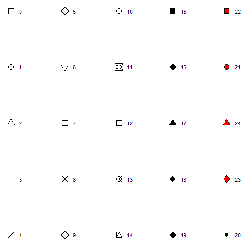
```
![](rvisualisation_files/figure-html/unnamed-chunk-28-1.png)
]
.pull-right[
![](rvisualisation_files/figure-html/unnamed-chunk-29-1.png)
]
---
.pull-left[
### позиционирование параметров
```r
wc3_units %>% 
 ggplot(aes(race, hp, color = armor_type)) +
* geom_point(aes(shape = air_attack, 
* size = armor, alpha = sight))
```
 - **shape**, **size** и **alpha** появились в легенде
]
.pull-right[
![](rvisualisation_files/figure-html/unnamed-chunk-30-1.png)
]
---
# Типы геометрий
Чтобы увидеть все доступные типы геометрий с описанием введите в консоли:

```r
??geom_
```
Или начните вводить **geom_** и нажмите **Tab**
---
<img src="img/geoms.png">
---
 Перед тем как начать подробно рассматривать геометрии
 Для построения графиков нам нужно будет модифицировать данные
 Мы рассмотрим два способа:
 - **stat_summary()** внутри ggplot 
 - подготовка данных при помощи **dplyr** (group_by(), summarise(), pivot_longer()) 
 
 
 Примеры будут по ходу лекции

---

.pull-left[
### geom_point()
```r
ggplot(data = wc3_units, 
 aes(x = gold, y = hp)) +
* geom_point()
```
 **geom_point()** - отрисовывает переменные, поданные в аэстетики (aes), в виде точек. Получилась обычная диаграмма рассеяния!

geom_point(
 mapping = NULL,
 data = NULL,
 stat = "identity",
 position = "identity",
 ...,
 na.rm = FALSE,
 show.legend = NA,
 inherit.aes = TRUE
 )

]
.pull-right[
![](rvisualisation_files/figure-html/unnamed-chunk-32-1.png)
]

---

.pull-left[
### geom_point()
```r
wc3_units %>% 
 ggplot(aes(x = damage, y = gold))+
 geom_point(size = 4)
```
Построим зависимость damage от gold
]
.pull-right[
![](rvisualisation_files/figure-html/unnamed-chunk-33-1.png)

]
---
.pull-left[
### geom_smooth()
```r
wc3_units %>% 
 ggplot(aes(x = damage, y = gold))+
 geom_point(size = 4)+
* geom_smooth()
```
 Добавим регрессионную линию с помощью geom_smooth()
 По умолчанию линия не прямая, пытается максимально приблизить точки.
]
.pull-right[

```
## `geom_smooth()` using method = 'loess' and formula = 'y ~ x'
```

![](rvisualisation_files/figure-html/unnamed-chunk-34-1.png)

]
---
.pull-left[
### geom_smooth()
```r
wc3_units %>% 
 ggplot(aes(x = damage, y = gold))+
 geom_point(size = 4)+
* geom_smooth(method = 'lm')
```
 Добавим регрессионную прямую с помощью geom_smooth(method = 'lm')
]
.pull-right[

```
## `geom_smooth()` using formula = 'y ~ x'
```

![](rvisualisation_files/figure-html/unnamed-chunk-35-1.png)

]
---
.pull-left[
### geom_smooth()
```r
wc3_units %>% 
 ggplot(aes(x = damage, y = gold, 
* color = race))+
 geom_point(size = 4)+
 geom_smooth(method = 'lm')
```
 Добавим race юнитов с помощью цвета color в aes()

Обратите внимание, как прописываются aesthetics. В функции ggplot() применяются на всем графике, на всех geoms, поэтому geom_smooth() строит регрессию отдельно по каждой расе. 
 Если бы мы хотели построить регрессию по всему датасету, то аэстетику цвета нужно было бы прописать отдельно в geom_point()
]
.pull-right[

```
## `geom_smooth()` using formula = 'y ~ x'
```

![](rvisualisation_files/figure-html/unnamed-chunk-36-1.png)

]
---
.pull-left[
### geom_smooth()
```r
wc3_units %>% 
 ggplot(aes(x = damage, y = gold))+
* geom_point(aes(color = race), 
 size = 4)+
 geom_smooth(method = 'lm')
```
 Если бы мы хотели построить регрессию по всему датасету, то аэстетику цвета нужно было бы прописать отдельно в geom_point()
]
.pull-right[

```
## `geom_smooth()` using formula = 'y ~ x'
```

![](rvisualisation_files/figure-html/unnamed-chunk-37-1.png)

]
---
.pull-left[
### geom_histogram()
```r
wc3_units %>% 
 ggplot(aes(hp)) +
* geom_histogram()
```
По умолчанию по оси у отложено количество наблюдений в диапазоне, определенном параметром bins или binwidth
]
.pull-right[
![](rvisualisation_files/figure-html/unnamed-chunk-38-1.png)
]
---
.pull-left[
### geom_histogram() 
### bins
```r
wc3_units %>% 
 ggplot(aes(hp)) +
* geom_histogram(bins = 5)
```
bins определяет количество долей на которые будут разделены данные
]
.pull-right[
![](rvisualisation_files/figure-html/unnamed-chunk-39-1.png)
]
---
.pull-left[
### geom_histogram() 
### binwidth
```r
wc3_units %>% 
 ggplot(aes(hp)) +
* geom_histogram(binwidth = 20)
```
binwidth определяет какого размера будут bins
]
.pull-right[
![](rvisualisation_files/figure-html/unnamed-chunk-40-1.png)
]
---
.pull-left[
### geom_histogram()
```r
wc3_units %>% 
 ggplot(aes(hp)) +
 geom_histogram(binwidth = 40,
* colour = 4, fill = "white")
```
]
.pull-right[
![](rvisualisation_files/figure-html/unnamed-chunk-41-1.png)
]
---
.pull-left[
### geom_boxplot()
```r
wc3_units %>%
 ggplot(aes(race, hp)) +
* geom_boxplot()
```
В описании к geom_boxplot() отмечено что подсчет статистик для него отличается от baser функции boxplot()
<img src="img/bp.png">
]
.pull-right[
![](rvisualisation_files/figure-html/unnamed-chunk-42-1.png)
]
---
.pull-left[
### geom_violin()
```r
wc3_units %>%
 ggplot(aes(race, hp)) +
* geom_violin()
```
<img src="img/v.png">
]
.pull-right[
![](rvisualisation_files/figure-html/unnamed-chunk-43-1.png)
]
---
.pull-left[
### geom_violin()
```r
wc3_units %>%
 ggplot(aes(race, hp)) +
 geom_violin()+
* geom_boxplot(width=0.1)
```
]
.pull-right[
![](rvisualisation_files/figure-html/unnamed-chunk-44-1.png)
]
---
.pull-left[
### geom_violin()
```r
wc3_units %>%
 ggplot(aes(race, hp)) +
 geom_violin()+
* geom_dotplot(binaxis='y', 
* stackdir='center', dotsize=1)
```
]
.pull-right[
![](rvisualisation_files/figure-html/unnamed-chunk-45-1.png)
]
---
.pull-left[
### geom_bar()
```r
wc3_units %>% 
 ggplot(aes(hp)) +
* geom_bar()
```
]
.pull-right[
![](rvisualisation_files/figure-html/unnamed-chunk-46-1.png)
по умолчанию параметр stat = "count"
]
---
.pull-left[
### geom_bar()
Приведем таблицу к виду:

```r
wc3_units %>% 
  group_by(race) %>%
  summarise(mean_hp=mean(hp))
```

```
## # A tibble: 4 × 2
## race mean_hp
## <chr> <dbl>
## 1 Human 556.
## 2 N.Elf 649.
## 3 Orc 483.
## 4 Undead 518.
```
и построим график
```r
wc3_units %>% 
 group_by(race) %>%
 summarise(mean_hp=mean(hp)) %>%
 ggplot(aes(race, mean_hp)) +
* geom_bar(stat = "identity")
```

]
.pull-right[
Чтобы посмотреть на средние значения по расе:
![](rvisualisation_files/figure-html/unnamed-chunk-48-1.png)
]
---

```r
wc3_units %>% 
 group_by(race) %>%
 summarise(mean_hp=mean(hp)) %>%
 ggplot(aes(race, mean_hp, 
* fill=mean_hp)) +
 geom_bar(stat = "identity") +
* scale_fill_gradient2(low="blue", high="red", 
* midpoint = 550)
```
 scale_fill_gradient позволяет выставить градиент

]
.pull-right[
![](rvisualisation_files/figure-html/unnamed-chunk-49-1.png)
]
---
.pull-left[
### geom_bar()

```r
* library(viridis)
wc3_units %>% 
 group_by(race) %>%
 summarise(mean_hp=mean(hp)) %>%
 ggplot(aes(race, mean_hp, 
 fill=mean_hp)) +
 geom_bar(stat = "identity") +
* scale_fill_viridis()
```
 scale_fill_gradient позволяет выставить градиент

]
.pull-right[

```
## Loading required package: viridisLite
```

![](rvisualisation_files/figure-html/unnamed-chunk-50-1.png)
]
---
.pull-left[
### stat_summary()
```r
wc3_units %>% 
 ggplot(aes(race, hp)) +
* stat_summary(geom = "bar", fun="mean")
```
<img src="img/sumf.png">
]
.pull-right[
![](rvisualisation_files/figure-html/unnamed-chunk-51-1.png)
то же самое можно задать при помощи **stat_summary()**
]
---

.pull-left[
### stat_summary()
```r
wc3_units %>% 
 ggplot(aes(race, hp)) +
 stat_summary(geom = "bar", fun="mean")+
* stat_summary(geom = "errorbar", 
* fun.data="mean_se", width = 0.2)
```
]
.pull-right[
![](rvisualisation_files/figure-html/unnamed-chunk-52-1.png)
дорисуем усы со стандартной ошибкой среднего
]
---

.pull-left[
### Надстройки
```r
wc3_units %>% 
 ggplot(aes(race, hp)) +
 stat_summary(geom = "bar", fun="mean")+
 stat_summary(geom = "errorbar", 
 fun.data="mean_se", width = 0.2)+
* geom_point()
```
 
 на основе этого кода потренируемся создавать сложные графики
 На одном плоте можно рисовать несколько геометрий
]
.pull-right[
![](rvisualisation_files/figure-html/unnamed-chunk-53-1.png)
]
---
.pull-left[
### position_jitterdodge()
```r
wc3_units %>% 
 ggplot(aes(race, hp)) +
 stat_summary(geom = "bar", fun="mean")+
 stat_summary(geom = "errorbar", 
 fun.data="mean_se", width = 0.2)+
 geom_point(aes(color=armor_type),
* position = position_jitterdodge(seed=1))
```
 Фиксация генератора случайных чисел:
 Для воспроизводимости положения точек мы указываем **seed** (для создания списка "рандомных" позиций)

]
.pull-right[
![](rvisualisation_files/figure-html/unnamed-chunk-54-1.png)
]
---
.pull-left[
### geom_text()
```r
plt <- 
wc3_units %>% 
 ggplot(aes(race, hp)) +
 stat_summary(geom = "bar", fun="mean")+
 stat_summary(geom = "errorbar", 
 fun.data="mean_se", width = 0.2)+
 geom_point(aes(color=armor_type),
 position = position_jitterdodge(seed=1))+
* geom_text(aes(label = unit,color=armor_type), 
* position = position_jitterdodge(seed = 1), 
* size = 3)
```
Чтобы позиции текста и точек совпали на графике необходимо чтобы **seed** указанный для geom_point() соответствовал значению **seed** у geom_text()
]
.pull-right[
![](rvisualisation_files/figure-html/unnamed-chunk-55-1.png)

]
---
.pull-left[
### theme_()
```r
plt + 
*  ggtitle("Title") +
*  xlab("x") +
*  ylab("y") +
*  theme_dark()
```
сохраним в переменную plt

```r
#??theme
```
[base r themes](https://ggplot2.tidyverse.org/reference/ggtheme.html)
]
.pull-right[
![](rvisualisation_files/figure-html/unnamed-chunk-57-1.png)
]
---

.pull-left[
### theme()
```r
plt + 
  ggtitle("Title") +
  xlab("x") +
  ylab("y") +
*  theme(panel.border = element_rect(linetype = "dashed", fill = NA))

```
]
.pull-right[
![](rvisualisation_files/figure-html/unnamed-chunk-58-1.png)
]
---
.pull-left[
### theme()
```r
plt + 
 ggtitle("Title") +
 xlab("x") +
 ylab("y") +
* theme(axis.text = element_text(colour = "blue"))

```
]
.pull-right[
![](rvisualisation_files/figure-html/unnamed-chunk-59-1.png)
]
---

.pull-left[
### theme()
```r
plt + 
  ggtitle("Title") +
  xlab("x") +
  ylab("y") +
*  theme(axis.text.x = element_text(angle = 90, 
* vjust = 0.5, hjust=1))

```
]
.pull-right[
![](rvisualisation_files/figure-html/unnamed-chunk-60-1.png)
]
---

```
]
.pull-right[
![](rvisualisation_files/figure-html/unnamed-chunk-61-1.png)
]
---

.pull-left[
### scales
```r
plt + 
*  scale_y_continuous(limits = c(0,1500), 
*  breaks = seq(0, 1500, 300))

```
]
.pull-right[
![](rvisualisation_files/figure-html/unnamed-chunk-62-1.png)
]
---
.pull-left[
### facet_wrap()
```r
plt + 
 ggtitle("Title") +
 xlab("x") +
 ylab("y") +
 theme_bw() + 
* facet_wrap(~armor_type)
```
]
.pull-right[
![](rvisualisation_files/figure-html/unnamed-chunk-63-1.png)
]
---

.pull-left[
### facet_wrap()
```r
plt + 
 ggtitle("Title") +
 xlab("x") +
 ylab("y") +
 theme_bw() + 
 facet_wrap(~armor_type, 
* scales = "free")
```
]
.pull-right[
![](rvisualisation_files/figure-html/unnamed-chunk-64-1.png)
]
---

.pull-left[
### factor levels
```r
wc3_units %>% 
* mutate(armor_type = 
* factor(armor_type, 
* levels=c("Unarmored", "Light", "Medium",
* "Heavy", "Fort", "Invulnerable"))) %>%
 ggplot(aes(race, hp)) +
 stat_summary(geom = "bar", fun="mean")+
 stat_summary(geom = "errorbar", 
 fun.data="mean_se", width = 0.2)+
 geom_point(aes(color=armor_type),
 position = position_jitterdodge(seed=1))+
 ggtitle("Title") +
 xlab("x")+
 ylab("y")+ theme_bw() + 
 facet_wrap(~armor_type)
```
]
.pull-right[
![](rvisualisation_files/figure-html/unnamed-chunk-65-1.png)
]
---
# ggplotly()
 пакет для создания интерактивных графиков
 [plotly](https://plotly.com/r/getting-started/):

```r
install.packages("plotly")
```

**echarts4r** — один из основных конкурентов для plotly. Симпатичный, работает довольно плавно, синтаксис тоже пытается вписаться в логику tidyverse.
 **leaflet** — основной (но не единственный!) пакет для работы с картами. Leaflet — это очень популярная библиотека JavaScript, используемая во многих веб-приложениях, а пакет leaflet - это довольно понятный интерфейс к ней с широкими возможностями.
 **networkD3** — пакет для интерактивной визуализации сетей. Подходит для небольших сетей.
---

.pull-left[
### ggplotly()
```r
ggplotly(plt)
```
]
.pull-right[
<div class="plotly html-widget html-fill-item-overflow-hidden html-fill-item" id="htmlwidget-8f4a986cd5545c388636" style="width:504px;height:504px;"></div>
<script type="application/json" data-for="htmlwidget-8f4a986cd5545c388636">{"x":{"data":[{"orientation":"v","width":[0.9,0.9,0.9,0.9],"base":[0,0,0,0],"x":[1,2,3,4],"y":[307.5,432,537.5,333.333333333333],"text":["race: Human hp: 307.5000","race: N.Elf hp: 432.0000","race: Orc hp: 537.5000","race: Undead hp: 333.3333"],"type":"bar","textposition":"none","marker":{"autocolorscale":false,"color":"rgba(89,89,89,1)","line":{"width":1.88976377952756,"color":"transparent"}},"showlegend":false,"xaxis":"x","yaxis":"y","hoverinfo":"text","frame":null},{"orientation":"v","width":[0.9,0.9,0.9,0.9],"base":[0,0,0,0],"x":[1,2,3,4],"y":[883.333333333333,803.75,447.5,1125],"text":["race: Human hp: 883.3333","race: N.Elf hp: 803.7500","race: Orc hp: 447.5000","race: Undead hp: 1125.0000"],"type":"bar","textposition":"none","marker":{"autocolorscale":false,"color":"rgba(89,89,89,1)","line":{"width":1.88976377952756,"color":"transparent"}},"showlegend":false,"xaxis":"x2","yaxis":"y","hoverinfo":"text","frame":null},{"orientation":"v","width":[0.9,0.9,0.9,0.9],"base":[0,0,0,0],"x":[1,2,3,4],"y":[451.666666666667,891.25,415,281.25],"text":["race: Human hp: 451.6667","race: N.Elf hp: 891.2500","race: Orc hp: 415.0000","race: Undead hp: 281.2500"],"type":"bar","textposition":"none","marker":{"autocolorscale":false,"color":"rgba(89,89,89,1)","line":{"width":1.88976377952756,"color":"transparent"}},"showlegend":false,"xaxis":"x3","yaxis":"y","hoverinfo":"text","frame":null},{"orientation":"v","width":[0.9,0.9,0.9,0.9],"base":[0,0,0,0],"x":[1,2,3,4],"y":[516.875,578,500,550],"text":["race: Human hp: 516.8750","race: N.Elf hp: 578.0000","race: Orc hp: 500.0000","race: Undead hp: 550.0000"],"type":"bar","textposition":"none","marker":{"autocolorscale":false,"color":"rgba(89,89,89,1)","line":{"width":1.88976377952756,"color":"transparent"}},"showlegend":false,"xaxis":"x","yaxis":"y2","hoverinfo":"text","frame":null},{"orientation":"v","width":0.9,"base":0,"x":[1],"y":[700],"text":"race: Human hp: 700.0000","type":"bar","textposition":"none","marker":{"autocolorscale":false,"color":"rgba(89,89,89,1)","line":{"width":1.88976377952756,"color":"transparent"}},"showlegend":false,"xaxis":"x2","yaxis":"y2","hoverinfo":"text","frame":null},{"orientation":"v","width":0.9,"base":0,"x":[2],"y":[500],"text":"race: N.Elf hp: 500.0000","type":"bar","textposition":"none","marker":{"autocolorscale":false,"color":"rgba(89,89,89,1)","line":{"width":1.88976377952756,"color":"transparent"}},"showlegend":false,"xaxis":"x3","yaxis":"y2","hoverinfo":"text","frame":null},{"x":[1,2,3,4],"y":[307.5,432,537.5,333.333333333333],"text":["race: Human hp: NA","race: N.Elf hp: NA","race: Orc hp: NA","race: Undead hp: NA"],"type":"scatter","mode":"lines","opacity":1,"line":{"color":"transparent"},"error_y":{"array":[17.5,59.8873943330314,159.641525508455,38.7656778320434],"arrayminus":[17.5,59.8873943330314,159.641525508455,38.7656778320434],"type":"data","width":8.00000000000001,"symmetric":false,"color":"rgba(0,0,0,1)"},"showlegend":false,"xaxis":"x","yaxis":"y","hoverinfo":"text","frame":null},{"x":[1,2,3,4],"y":[883.333333333333,803.75,447.5,1125],"text":["race: Human hp: NA","race: N.Elf hp: NA","race: Orc hp: NA","race: Undead hp: NA"],"type":"scatter","mode":"lines","opacity":1,"line":{"color":"transparent"},"error_y":{"array":[197.026506958948,130.278147950197,122.5,225],"arrayminus":[197.026506958948,130.278147950197,122.5,225],"type":"data","width":8.00000000000001,"symmetric":false,"color":"rgba(0,0,0,1)"},"showlegend":false,"xaxis":"x2","yaxis":"y","hoverinfo":"text","frame":null},{"x":[1,2,3,4],"y":[451.666666666667,891.25,415,281.25],"text":["race: Human hp: NA","race: N.Elf hp: NA","race: Orc hp: NA","race: Undead hp: NA"],"type":"scatter","mode":"lines","opacity":1,"line":{"color":"transparent"},"error_y":{"array":[117.34327609388,409.991742803031,76.7571929311297,92.6547129580214],"arrayminus":[117.34327609388,409.991742803031,76.7571929311297,92.6547129580214],"type":"data","width":8.00000000000001,"symmetric":false,"color":"rgba(0,0,0,1)"},"showlegend":false,"xaxis":"x3","yaxis":"y","hoverinfo":"text","frame":null},{"x":[1,2,3,4],"y":[516.875,578,500,550],"text":["race: Human hp: NA","race: N.Elf hp: NA","race: Orc hp: NA","race: Undead hp: NA"],"type":"scatter","mode":"lines","opacity":1,"line":{"color":"transparent"},"error_y":{"array":[94.0741420180304,210.722566423248,154.013759434792,156.62898483004],"arrayminus":[94.0741420180305,210.722566423248,154.013759434792,156.62898483004],"type":"data","width":8.00000000000001,"symmetric":false,"color":"rgba(0,0,0,1)"},"showlegend":false,"xaxis":"x","yaxis":"y2","hoverinfo":"text","frame":null},{"x":[1],"y":[700],"text":"race: Human hp: 700","type":"scatter","mode":"lines","opacity":1,"line":{"color":"transparent"},"error_y":{"array":[null],"arrayminus":[null],"type":"data","width":8.00000000000001,"symmetric":false,"color":"rgba(0,0,0,1)"},"showlegend":false,"xaxis":"x2","yaxis":"y2","hoverinfo":"text","frame":null},{"x":[2],"y":[500],"text":"race: N.Elf hp: 500","type":"scatter","mode":"lines","opacity":1,"line":{"color":"transparent"},"error_y":{"array":[null],"arrayminus":[null],"type":"data","width":8.00000000000001,"symmetric":false,"color":"rgba(0,0,0,1)"},"showlegend":false,"xaxis":"x3","yaxis":"y2","hoverinfo":"text","frame":null},{"x":[0.97655086631421,0.987212389963679,3.00728533633519,3.04082077899948,2.97016819310375,3.03983896849677,2.04446752686054,2.01607977924868,2.01291140438989,1.95617862704676,1.97059745748993,3.9676556752529,4.01870228466578,3.98841037182137],"y":[290,325,335,315,500,1000,600,435,525,300,300,410,305,285],"text":["race: Human hp: 290 armor_type: Unarmored","race: Human hp: 325 armor_type: Unarmored","race: Orc hp: 335 armor_type: Unarmored","race: Orc hp: 315 armor_type: Unarmored","race: Orc hp: 500 armor_type: Unarmored","race: Orc hp: 1000 armor_type: Unarmored","race: N.Elf hp: 600 armor_type: Unarmored","race: N.Elf hp: 435 armor_type: Unarmored","race: N.Elf hp: 525 armor_type: Unarmored","race: N.Elf hp: 300 armor_type: Unarmored","race: N.Elf hp: 300 armor_type: Unarmored","race: Undead hp: 410 armor_type: Unarmored","race: Undead hp: 305 armor_type: Unarmored","race: Undead hp: 285 armor_type: Unarmored"],"type":"scatter","mode":"markers","marker":{"autocolorscale":false,"color":"rgba(248,118,109,1)","opacity":1,"size":5.66929133858268,"symbol":"circle","line":{"width":1.88976377952756,"color":"rgba(248,118,109,1)"}},"hoveron":"points","name":"Unarmored","legendgroup":"Unarmored","showlegend":true,"xaxis":"x","yaxis":"y","hoverinfo":"text","frame":null},{"x":[0.97655086631421,0.987212389963679,1.00728533633519,3.04082077899948,2.97016819310375,2.03983896849677,2.04446752686054,2.01607977924868,2.01291140438989,3.95617862704676,3.97059745748993],"y":[825,575,1250,570,325,450,765,1000,1000,1350,900],"text":["race: Human hp: 825 armor_type: Light","race: Human hp: 575 armor_type: Light","race: Human hp: 1250 armor_type: Light","race: Orc hp: 570 armor_type: Light","race: Orc hp: 325 armor_type: Light","race: N.Elf hp: 450 armor_type: Light","race: N.Elf hp: 765 armor_type: Light","race: N.Elf hp: 1000 armor_type: Light","race: N.Elf hp: 1000 armor_type: Light","race: Undead hp: 1350 armor_type: Light","race: Undead hp: 900 armor_type: Light"],"type":"scatter","mode":"markers","marker":{"autocolorscale":false,"color":"rgba(183,159,0,1)","opacity":1,"size":5.66929133858268,"symbol":"circle","line":{"width":1.88976377952756,"color":"rgba(183,159,0,1)"}},"hoveron":"points","name":"Light","legendgroup":"Light","showlegend":true,"xaxis":"x2","yaxis":"y","hoverinfo":"text","frame":null},{"x":[0.97655086631421,0.987212389963679,1.00728533633519,3.04082077899948,2.97016819310375,3.03983896849677,3.04446752686054,2.01607977924868,2.01291140438989,1.95617862704676,1.97059745748993,3.9676556752529,4.01870228466578,3.98841037182137,4.02698414199986],"y":[220,535,600,250,350,450,610,120,245,1600,1600,220,550,125,230],"text":["race: Human hp: 220 armor_type: Medium","race: Human hp: 535 armor_type: Medium","race: Human hp: 600 armor_type: Medium","race: Orc hp: 250 armor_type: Medium","race: Orc hp: 350 armor_type: Medium","race: Orc hp: 450 armor_type: Medium","race: Orc hp: 610 armor_type: Medium","race: N.Elf hp: 120 armor_type: Medium","race: N.Elf hp: 245 armor_type: Medium","race: N.Elf hp: 1600 armor_type: Medium","race: N.Elf hp: 1600 armor_type: Medium","race: Undead hp: 220 armor_type: Medium","race: Undead hp: 550 armor_type: Medium","race: Undead hp: 125 armor_type: Medium","race: Undead hp: 230 armor_type: Medium"],"type":"scatter","mode":"markers","marker":{"autocolorscale":false,"color":"rgba(0,186,56,1)","opacity":1,"size":5.66929133858268,"symbol":"circle","line":{"width":1.88976377952756,"color":"rgba(0,186,56,1)"}},"hoveron":"points","name":"Medium","legendgroup":"Medium","showlegend":true,"xaxis":"x3","yaxis":"y","hoverinfo":"text","frame":null},{"x":[0.97655086631421,0.987212389963679,1.00728533633519,1.04082077899948,0.970168193103746,1.03983896849677,1.04446752686054,1.01607977924868,3.01291140438989,2.95617862704676,2.97059745748993,2.9676556752529,3.01870228466578,2.98841037182137,3.02698414199986,1.99976992420852,2.02176185082644,2.04919060948305,1.98800351794343,2.02774452213198,4.04347052311059,3.97121425212827,4.01516737660859,3.96255550959613,3.97672206687275,3.98861140925437,3.95133903331589,3.988238795707,4.03696908457205],"y":[220,420,835,200,360,525,675,900,700,425,1300,200,300,500,75,300,130,960,300,1200,340,1175,380,180,1500,140,275,410,550],"text":["race: Human hp: 220 armor_type: Heavy","race: Human hp: 420 armor_type: Heavy","race: Human hp: 835 armor_type: Heavy","race: Human hp: 200 armor_type: Heavy","race: Human hp: 360 armor_type: Heavy","race: Human hp: 525 armor_type: Heavy","race: Human hp: 675 armor_type: Heavy","race: Human hp: 900 armor_type: Heavy","race: Orc hp: 700 armor_type: Heavy","race: Orc hp: 425 armor_type: Heavy","race: Orc hp: 1300 armor_type: Heavy","race: Orc hp: 200 armor_type: Heavy","race: Orc hp: 300 armor_type: Heavy","race: Orc hp: 500 armor_type: Heavy","race: Orc hp: 75 armor_type: Heavy","race: N.Elf hp: 300 armor_type: Heavy","race: N.Elf hp: 130 armor_type: Heavy","race: N.Elf hp: 960 armor_type: Heavy","race: N.Elf hp: 300 armor_type: Heavy","race: N.Elf hp: 1200 armor_type: Heavy","race: Undead hp: 340 armor_type: Heavy","race: Undead hp: 1175 armor_type: Heavy","race: Undead hp: 380 armor_type: Heavy","race: Undead hp: 180 armor_type: Heavy","race: Undead hp: 1500 armor_type: Heavy","race: Undead hp: 140 armor_type: Heavy","race: Undead hp: 275 armor_type: Heavy","race: Undead hp: 410 armor_type: Heavy","race: Undead hp: 550 armor_type: Heavy"],"type":"scatter","mode":"markers","marker":{"autocolorscale":false,"color":"rgba(0,191,196,1)","opacity":1,"size":5.66929133858268,"symbol":"circle","line":{"width":1.88976377952756,"color":"rgba(0,191,196,1)"}},"hoveron":"points","name":"Heavy","legendgroup":"Heavy","showlegend":true,"xaxis":"x","yaxis":"y2","hoverinfo":"text","frame":null},{"x":[0.97655086631421],"y":[700],"text":"race: Human hp: 700 armor_type: Fort","type":"scatter","mode":"markers","marker":{"autocolorscale":false,"color":"rgba(97,156,255,1)","opacity":1,"size":5.66929133858268,"symbol":"circle","line":{"width":1.88976377952756,"color":"rgba(97,156,255,1)"}},"hoveron":"points","name":"Fort","legendgroup":"Fort","showlegend":true,"xaxis":"x2","yaxis":"y2","hoverinfo":"text","frame":null},{"x":[1.97655086631421],"y":[500],"text":"race: N.Elf hp: 500 armor_type: Invulnerable","type":"scatter","mode":"markers","marker":{"autocolorscale":false,"color":"rgba(245,100,227,1)","opacity":1,"size":5.66929133858268,"symbol":"circle","line":{"width":1.88976377952756,"color":"rgba(245,100,227,1)"}},"hoveron":"points","name":"Invulnerable","legendgroup":"Invulnerable","showlegend":true,"xaxis":"x3","yaxis":"y2","hoverinfo":"text","frame":null}],"layout":{"margin":{"t":52.5296803652968,"r":7.30593607305936,"b":37.2602739726027,"l":48.9497716894977},"plot_bgcolor":"rgba(255,255,255,1)","paper_bgcolor":"rgba(255,255,255,1)","font":{"color":"rgba(0,0,0,1)","family":"","size":14.6118721461187},"title":{"text":"Title","font":{"color":"rgba(0,0,0,1)","family":"","size":17.5342465753425},"x":0,"xref":"paper"},"xaxis":{"domain":[0,0.322461404653185],"automargin":true,"type":"linear","autorange":false,"range":[0.4,4.6],"tickmode":"array","ticktext":["Human","N.Elf","Orc","Undead"],"tickvals":[1,2,3,4],"categoryorder":"array","categoryarray":["Human","N.Elf","Orc","Undead"],"nticks":null,"ticks":"outside","tickcolor":"rgba(51,51,51,1)","ticklen":3.65296803652968,"tickwidth":0.66417600664176,"showticklabels":true,"tickfont":{"color":"rgba(77,77,77,1)","family":"","size":11.689497716895},"tickangle":-0,"showline":false,"linecolor":null,"linewidth":0,"showgrid":true,"gridcolor":"rgba(235,235,235,1)","gridwidth":0.66417600664176,"zeroline":false,"anchor":"y2","title":"","hoverformat":".2f"},"annotations":[{"text":"x","x":0.5,"y":0,"showarrow":false,"ax":0,"ay":0,"font":{"color":"rgba(0,0,0,1)","family":"","size":14.6118721461187},"xref":"paper","yref":"paper","textangle":-0,"xanchor":"center","yanchor":"top","annotationType":"axis","yshift":-21.9178082191781},{"text":"y","x":0,"y":0.5,"showarrow":false,"ax":0,"ay":0,"font":{"color":"rgba(0,0,0,1)","family":"","size":14.6118721461187},"xref":"paper","yref":"paper","textangle":-90,"xanchor":"right","yanchor":"center","annotationType":"axis","xshift":-33.6073059360731},{"text":"Unarmored","x":0.161230702326593,"y":1,"showarrow":false,"ax":0,"ay":0,"font":{"color":"rgba(26,26,26,1)","family":"","size":11.689497716895},"xref":"paper","yref":"paper","textangle":-0,"xanchor":"center","yanchor":"bottom"},{"text":"Light","x":0.5,"y":1,"showarrow":false,"ax":0,"ay":0,"font":{"color":"rgba(26,26,26,1)","family":"","size":11.689497716895},"xref":"paper","yref":"paper","textangle":-0,"xanchor":"center","yanchor":"bottom"},{"text":"Medium","x":0.838769297673407,"y":1,"showarrow":false,"ax":0,"ay":0,"font":{"color":"rgba(26,26,26,1)","family":"","size":11.689497716895},"xref":"paper","yref":"paper","textangle":-0,"xanchor":"center","yanchor":"bottom"},{"text":"Heavy","x":0.161230702326593,"y":0.471732985431616,"showarrow":false,"ax":0,"ay":0,"font":{"color":"rgba(26,26,26,1)","family":"","size":11.689497716895},"xref":"paper","yref":"paper","textangle":-0,"xanchor":"center","yanchor":"bottom"},{"text":"Fort","x":0.5,"y":0.471732985431616,"showarrow":false,"ax":0,"ay":0,"font":{"color":"rgba(26,26,26,1)","family":"","size":11.689497716895},"xref":"paper","yref":"paper","textangle":-0,"xanchor":"center","yanchor":"bottom"},{"text":"Invulnerable","x":0.838769297673407,"y":0.471732985431616,"showarrow":false,"ax":0,"ay":0,"font":{"color":"rgba(26,26,26,1)","family":"","size":11.689497716895},"xref":"paper","yref":"paper","textangle":-0,"xanchor":"center","yanchor":"bottom"}],"yaxis":{"domain":[0.528267014568384,1],"automargin":true,"type":"linear","autorange":false,"range":[-80,1680],"tickmode":"array","ticktext":["0","500","1000","1500"],"tickvals":[0,500,1000,1500],"categoryorder":"array","categoryarray":["0","500","1000","1500"],"nticks":null,"ticks":"outside","tickcolor":"rgba(51,51,51,1)","ticklen":3.65296803652968,"tickwidth":0.66417600664176,"showticklabels":true,"tickfont":{"color":"rgba(77,77,77,1)","family":"","size":11.689497716895},"tickangle":-0,"showline":false,"linecolor":null,"linewidth":0,"showgrid":true,"gridcolor":"rgba(235,235,235,1)","gridwidth":0.66417600664176,"zeroline":false,"anchor":"x","title":"","hoverformat":".2f"},"shapes":[{"type":"rect","fillcolor":"transparent","line":{"color":"rgba(51,51,51,1)","width":0.66417600664176,"linetype":"solid"},"yref":"paper","xref":"paper","x0":0,"x1":0.322461404653185,"y0":0.528267014568384,"y1":1},{"type":"rect","fillcolor":"rgba(217,217,217,1)","line":{"color":"rgba(51,51,51,1)","width":0.66417600664176,"linetype":"solid"},"yref":"paper","xref":"paper","x0":0,"x1":0.322461404653185,"y0":0,"y1":23.37899543379,"yanchor":1,"ysizemode":"pixel"},{"type":"rect","fillcolor":"transparent","line":{"color":"rgba(51,51,51,1)","width":0.66417600664176,"linetype":"solid"},"yref":"paper","xref":"paper","x0":0.344205262013481,"x1":0.655794737986519,"y0":0.528267014568384,"y1":1},{"type":"rect","fillcolor":"rgba(217,217,217,1)","line":{"color":"rgba(51,51,51,1)","width":0.66417600664176,"linetype":"solid"},"yref":"paper","xref":"paper","x0":0.344205262013481,"x1":0.655794737986519,"y0":0,"y1":23.37899543379,"yanchor":1,"ysizemode":"pixel"},{"type":"rect","fillcolor":"transparent","line":{"color":"rgba(51,51,51,1)","width":0.66417600664176,"linetype":"solid"},"yref":"paper","xref":"paper","x0":0.677538595346814,"x1":1,"y0":0.528267014568384,"y1":1},{"type":"rect","fillcolor":"rgba(217,217,217,1)","line":{"color":"rgba(51,51,51,1)","width":0.66417600664176,"linetype":"solid"},"yref":"paper","xref":"paper","x0":0.677538595346814,"x1":1,"y0":0,"y1":23.37899543379,"yanchor":1,"ysizemode":"pixel"},{"type":"rect","fillcolor":"transparent","line":{"color":"rgba(51,51,51,1)","width":0.66417600664176,"linetype":"solid"},"yref":"paper","xref":"paper","x0":0,"x1":0.322461404653185,"y0":0,"y1":0.471732985431616},{"type":"rect","fillcolor":"rgba(217,217,217,1)","line":{"color":"rgba(51,51,51,1)","width":0.66417600664176,"linetype":"solid"},"yref":"paper","xref":"paper","x0":0,"x1":0.322461404653185,"y0":0,"y1":23.37899543379,"yanchor":0.471732985431616,"ysizemode":"pixel"},{"type":"rect","fillcolor":"transparent","line":{"color":"rgba(51,51,51,1)","width":0.66417600664176,"linetype":"solid"},"yref":"paper","xref":"paper","x0":0.344205262013481,"x1":0.655794737986519,"y0":0,"y1":0.471732985431616},{"type":"rect","fillcolor":"rgba(217,217,217,1)","line":{"color":"rgba(51,51,51,1)","width":0.66417600664176,"linetype":"solid"},"yref":"paper","xref":"paper","x0":0.344205262013481,"x1":0.655794737986519,"y0":0,"y1":23.37899543379,"yanchor":0.471732985431616,"ysizemode":"pixel"},{"type":"rect","fillcolor":"transparent","line":{"color":"rgba(51,51,51,1)","width":0.66417600664176,"linetype":"solid"},"yref":"paper","xref":"paper","x0":0.677538595346814,"x1":1,"y0":0,"y1":0.471732985431616},{"type":"rect","fillcolor":"rgba(217,217,217,1)","line":{"color":"rgba(51,51,51,1)","width":0.66417600664176,"linetype":"solid"},"yref":"paper","xref":"paper","x0":0.677538595346814,"x1":1,"y0":0,"y1":23.37899543379,"yanchor":0.471732985431616,"ysizemode":"pixel"}],"xaxis2":{"type":"linear","autorange":false,"range":[0.4,4.6],"tickmode":"array","ticktext":["Human","N.Elf","Orc","Undead"],"tickvals":[1,2,3,4],"categoryorder":"array","categoryarray":["Human","N.Elf","Orc","Undead"],"nticks":null,"ticks":"outside","tickcolor":"rgba(51,51,51,1)","ticklen":3.65296803652968,"tickwidth":0.66417600664176,"showticklabels":true,"tickfont":{"color":"rgba(77,77,77,1)","family":"","size":11.689497716895},"tickangle":-0,"showline":false,"linecolor":null,"linewidth":0,"showgrid":true,"domain":[0.344205262013481,0.655794737986519],"gridcolor":"rgba(235,235,235,1)","gridwidth":0.66417600664176,"zeroline":false,"anchor":"y2","title":"","hoverformat":".2f"},"xaxis3":{"type":"linear","autorange":false,"range":[0.4,4.6],"tickmode":"array","ticktext":["Human","N.Elf","Orc","Undead"],"tickvals":[1,2,3,4],"categoryorder":"array","categoryarray":["Human","N.Elf","Orc","Undead"],"nticks":null,"ticks":"outside","tickcolor":"rgba(51,51,51,1)","ticklen":3.65296803652968,"tickwidth":0.66417600664176,"showticklabels":true,"tickfont":{"color":"rgba(77,77,77,1)","family":"","size":11.689497716895},"tickangle":-0,"showline":false,"linecolor":null,"linewidth":0,"showgrid":true,"domain":[0.677538595346814,1],"gridcolor":"rgba(235,235,235,1)","gridwidth":0.66417600664176,"zeroline":false,"anchor":"y2","title":"","hoverformat":".2f"},"yaxis2":{"type":"linear","autorange":false,"range":[-80,1680],"tickmode":"array","ticktext":["0","500","1000","1500"],"tickvals":[0,500,1000,1500],"categoryorder":"array","categoryarray":["0","500","1000","1500"],"nticks":null,"ticks":"outside","tickcolor":"rgba(51,51,51,1)","ticklen":3.65296803652968,"tickwidth":0.66417600664176,"showticklabels":true,"tickfont":{"color":"rgba(77,77,77,1)","family":"","size":11.689497716895},"tickangle":-0,"showline":false,"linecolor":null,"linewidth":0,"showgrid":true,"domain":[0,0.471732985431616],"gridcolor":"rgba(235,235,235,1)","gridwidth":0.66417600664176,"zeroline":false,"anchor":"x","title":"","hoverformat":".2f"},"showlegend":true,"legend":{"bgcolor":"rgba(255,255,255,1)","bordercolor":"transparent","borderwidth":1.88976377952756,"font":{"color":"rgba(0,0,0,1)","family":"","size":11.689497716895},"title":{"text":"armor_type","font":{"color":"rgba(0,0,0,1)","family":"","size":14.6118721461187}}},"hovermode":"closest","barmode":"relative"},"config":{"doubleClick":"reset","modeBarButtonsToAdd":["hoverclosest","hovercompare"],"showSendToCloud":false},"source":"A","attrs":{"6da850283e80":{"x":{},"y":{},"type":"bar"},"6da8453b57b3":{"x":{},"y":{}},"6da83d4531a":{"x":{},"y":{},"colour":{}}},"cur_data":"6da850283e80","visdat":{"6da850283e80":["function (y) ","x"],"6da8453b57b3":["function (y) ","x"],"6da83d4531a":["function (y) ","x"]},"highlight":{"on":"plotly_click","persistent":false,"dynamic":false,"selectize":false,"opacityDim":0.2,"selected":{"opacity":1},"debounce":0},"shinyEvents":["plotly_hover","plotly_click","plotly_selected","plotly_relayout","plotly_brushed","plotly_brushing","plotly_clickannotation","plotly_doubleclick","plotly_deselect","plotly_afterplot","plotly_sunburstclick"],"base_url":"https://plot.ly"},"evals":[],"jsHooks":[]}</script>
]
---
.pull-left[
### ggplotly()
```r
library(viridis)
plt2 <- wc3_units %>%
 ggplot(aes(text=unit,damage, hp)) +
 geom_point(aes(size=damage,color=dps)) +
 scale_color_viridis()
ggplotly(plt2)
```
]
.pull-right[
<div class="plotly html-widget html-fill-item-overflow-hidden html-fill-item" id="htmlwidget-3d471b43fa2a060b7f32" style="width:504px;height:504px;"></div>
<script type="application/json" data-for="htmlwidget-3d471b43fa2a060b7f32">{"x":{"data":[{"x":[5.5,12.5,12.5,21,34,8.5,11,14,7.5,58,50,50,19,20,35,45,68,7.5,19.5,25,25,80.5,25,33,8.5,12,19.5,18,40,14,11.5,16.5,21.5,12,null,17,17,44.5,18,20.5,36.5,34,41,null,12,null,15,17,75,50,16,30.5,16,9.5,13,28.5,19.5,36,79.5,8.5,11,104,null,14.5,11.5,54.5,8.5,16.5,24.5,7.5,20],"y":[220,220,420,535,835,290,325,600,200,360,700,825,575,525,675,900,1250,250,700,350,450,425,610,1300,335,315,500,1000,570,325,200,300,500,75,120,245,600,300,435,130,960,1600,1600,525,300,300,450,765,1000,1000,300,1200,500,220,340,550,410,1175,380,305,285,1350,125,180,230,1500,140,275,410,550,900],"text":["damage: 5.5 hp: 220 Peasant damage: 5.5 dps: 2.75","damage: 12.5 hp: 220 Militia damage: 12.5 dps: 10.42","damage: 12.5 hp: 420 Footman damage: 12.5 dps: 9.26","damage: 21.0 hp: 535 Rifleman damage: 21.0 dps: 14.00","damage: 34.0 hp: 835 Knight damage: 34.0 dps: 24.29","damage: 8.5 hp: 290 Priest damage: 8.5 dps: 4.25","damage: 11.0 hp: 325 Sorceress damage: 11.0 dps: 6.29","damage: 14.0 hp: 600 Spell Breaker damage: 14.0 dps: 7.37","damage: 7.5 hp: 200 Flying Machine damage: 7.5 dps: 3.00","damage: 58.0 hp: 360 Mortar Team damage: 58.0 dps: 16.57","damage: 50.0 hp: 700 Siege Engine damage: 50.0 dps: 23.81","damage: 50.0 hp: 825 Gryphon Rider damage: 50.0 dps: 22.73","damage: 19.0 hp: 575 Dragonhawk Rider damage: 19.0 dps: 10.86","damage: 20.0 hp: 525 Water Elemental 1 damage: 20.0 dps: 13.33","damage: 35.0 hp: 675 Water Elemental 2 damage: 35.0 dps: 23.33","damage: 45.0 hp: 900 Water Elemental 3 damage: 45.0 dps: 30.00","damage: 68.0 hp: 1250 Phoenix damage: 68.0 dps: 48.57","damage: 7.5 hp: 250 Peon damage: 7.5 dps: 2.50","damage: 19.5 hp: 700 Grunt damage: 19.5 dps: 12.19","damage: 25.0 hp: 350 T. Headhunter damage: 25.0 dps: 10.82","damage: 25.0 hp: 450 T. Berserker damage: 25.0 dps: 10.82","damage: 80.5 hp: 425 Demolisher damage: 80.5 dps: 17.89","damage: 25.0 hp: 610 Raider damage: 25.0 dps: 13.51","damage: 33.0 hp: 1300 Tauren damage: 33.0 dps: 17.37","damage: 8.5 hp: 335 Shaman damage: 8.5 dps: 4.05","damage: 12.0 hp: 315 Witch Doctor damage: 12.0 dps: 6.86","damage: 19.5 hp: 500 Spirit Walker damage: 19.5 dps: 11.14","damage: 18.0 hp: 1000 Kodo Beast damage: 18.0 dps: 12.50","damage: 40.0 hp: 570 Wind Rider damage: 40.0 dps: 20.00","damage: 14.0 hp: 325 Troll Batrider damage: 14.0 dps: 7.78","damage: 11.5 hp: 200 Spirit Wolf damage: 11.5 dps: 11.50","damage: 16.5 hp: 300 Dire Wolf damage: 16.5 dps: 16.50","damage: 21.5 hp: 500 Shadow Wolf damage: 21.5 dps: 21.50","damage: 12.0 hp: 75 Serpent Ward damage: 12.0 dps: 8.00","damage: NA hp: 120 Wisp damage: NA dps: NA","damage: 17.0 hp: 245 Archer damage: 17.0 dps: 11.33","damage: 17.0 hp: 600 Huntress damage: 17.0 dps: 9.44","damage: 44.5 hp: 300 Glaive Thrower damage: 44.5 dps: 12.71","damage: 18.0 hp: 435 Dryad damage: 18.0 dps: 9.00","damage: 20.5 hp: 130 DoC Druid Form damage: 20.5 dps: 13.67","damage: 36.5 hp: 960 DoC Bear Form damage: 36.5 dps: 24.33","damage: 34.0 hp: 1600 Mountain Giant damage: 34.0 dps: 13.60","damage: 41.0 hp: 1600 Mountain Giant 2 damage: 41.0 dps: 16.40","damage: NA hp: 525 Hippogryph damage: NA dps: NA","damage: 12.0 hp: 300 DoT Druid Form damage: 12.0 dps: 7.50","damage: NA hp: 300 DoT Crow Form damage: NA dps: NA","damage: 15.0 hp: 450 Faerie Dragon damage: 15.0 dps: 8.57","damage: 17.0 hp: 765 Hippogryph Rider damage: 17.0 dps: 15.45","damage: 75.0 hp: 1000 Chimaera damage: 75.0 dps: 30.00","damage: 50.0 hp: 1000 Chimaera 2 damage: 50.0 dps: 20.00","damage: 16.0 hp: 300 Treant damage: 16.0 dps: 9.14","damage: 30.5 hp: 1200 Avatar of Vengeance damage: 30.5 dps: 22.59","damage: 16.0 hp: 500 Spirit of Vengeance damage: 16.0 dps: 11.85","damage: 9.5 hp: 220 Acolyte damage: 9.5 dps: 3.80","damage: 13.0 hp: 340 Ghoul damage: 13.0 dps: 10.00","damage: 28.5 hp: 550 Crypt Fiend damage: 28.5 dps: 14.25","damage: 19.5 hp: 410 Gargoyle damage: 19.5 dps: 8.86","damage: 36.0 hp: 1175 Abomination damage: 36.0 dps: 18.95","damage: 79.5 hp: 380 Meat Wagon damage: 79.5 dps: 19.88","damage: 8.5 hp: 305 Necromancer damage: 8.5 dps: 4.72","damage: 11.0 hp: 285 Banshee damage: 11.0 dps: 7.33","damage: 104.0 hp: 1350 Frost Wyrm damage: 104.0 dps: 34.67","damage: NA hp: 125 Shade damage: NA dps: NA","damage: 14.5 hp: 180 Skeleton Warrior damage: 14.5 dps: 7.25","damage: 11.5 hp: 230 Skeletal Mage damage: 11.5 dps: 7.67","damage: 54.5 hp: 1500 Infernal damage: 54.5 dps: 40.37","damage: 8.5 hp: 140 Carrion Beetle 1 damage: 8.5 dps: 5.67","damage: 16.5 hp: 275 Carrion Beetle 2 damage: 16.5 dps: 11.00","damage: 24.5 hp: 410 Carrion Beetle 3 damage: 24.5 dps: 16.33","damage: 7.5 hp: 550 Obsidian Statue damage: 7.5 dps: 3.57","damage: 20.0 hp: 900 Destroyer damage: 20.0 dps: 14.81"],"type":"scatter","mode":"markers","marker":{"autocolorscale":false,"color":["rgba(68,3,86,1)","rgba(68,59,132,1)","rgba(70,51,127,1)","rgba(59,82,139,1)","rgba(35,138,141,1)","rgba(71,15,98,1)","rgba(72,31,112,1)","rgba(72,38,119,1)","rgba(69,5,89,1)","rgba(52,97,141,1)","rgba(36,135,142,1)","rgba(38,130,142,1)","rgba(67,62,133,1)","rgba(61,78,138,1)","rgba(37,132,142,1)","rgba(34,167,133,1)","rgba(253,231,37,1)","rgba(68,1,84,1)","rgba(63,71,136,1)","rgba(67,62,133,1)","rgba(67,62,133,1)","rgba(49,104,142,1)","rgba(60,79,138,1)","rgba(50,101,142,1)","rgba(71,14,97,1)","rgba(72,35,116,1)","rgba(66,64,134,1)","rgba(63,72,137,1)","rgba(44,115,142,1)","rgba(72,41,121,1)","rgba(65,66,135,1)","rgba(52,96,141,1)","rgba(41,123,142,1)","rgba(71,43,122,1)","rgba(127,127,127,1)","rgba(66,65,134,1)","rgba(70,52,128,1)","rgba(62,74,137,1)","rgba(70,50,126,1)","rgba(60,80,139,1)","rgba(35,138,141,1)","rgba(60,79,138,1)","rgba(52,96,141,1)","rgba(127,127,127,1)","rgba(72,39,120,1)","rgba(127,127,127,1)","rgba(71,47,125,1)","rgba(55,91,141,1)","rgba(34,167,133,1)","rgba(44,115,142,1)","rgba(70,51,127,1)","rgba(38,129,142,1)","rgba(64,69,136,1)","rgba(70,11,94,1)","rgba(68,57,131,1)","rgba(58,83,139,1)","rgba(70,48,126,1)","rgba(46,110,142,1)","rgba(44,114,142,1)","rgba(71,19,102,1)","rgba(72,38,119,1)","rgba(66,190,113,1)","rgba(127,127,127,1)","rgba(72,37,118,1)","rgba(72,41,121,1)","rgba(136,213,72,1)","rgba(72,27,109,1)","rgba(66,63,133,1)","rgba(52,96,141,1)","rgba(70,10,93,1)","rgba(57,86,140,1)"],"opacity":1,"size":[3.77952755905512,8.81729859917696,8.81729859917696,11.2759707567771,13.9446317746805,7.07752286265723,8.24503430985055,9.33088086829253,6.47232944836194,17.5760317501601,16.4814486670986,16.4814486670986,10.7756320895504,11.0301185424953,14.1214294500059,15.746600918792,18.8327477451299,6.47232944836194,10.9040116881258,12.1877987634574,12.1877987634574,20.2695040770657,12.1877987634574,13.7647042078179,7.07752286265723,8.63404520233614,10.9040116881258,10.5115322823222,14.9635737749686,9.33088086829253,8.443597246052,10.0947077688986,11.3959214643383,8.63404520233614,null,10.236639652442,10.236639652442,15.670618732432,10.5115322823222,11.1540692473845,14.381099198833,13.9446317746805,15.1245035734509,null,8.63404520233614,null,9.64835321428703,10.236639652442,19.653360587758,16.4814486670986,9.94951180368942,13.3000199406591,9.94951180368942,7.58772451169672,8.99411599501571,12.9112630552861,10.9040116881258,14.2952551006748,20.1592019928469,7.07752286265723,8.24503430985055,22.6771653543307,null,9.49182298801752,8.443597246052,17.1082168933007,7.07752286265723,10.0947077688986,12.0793003958873,6.47232944836194,11.0301185424953],"symbol":"circle","line":{"width":1.88976377952756,"color":["rgba(68,3,86,1)","rgba(68,59,132,1)","rgba(70,51,127,1)","rgba(59,82,139,1)","rgba(35,138,141,1)","rgba(71,15,98,1)","rgba(72,31,112,1)","rgba(72,38,119,1)","rgba(69,5,89,1)","rgba(52,97,141,1)","rgba(36,135,142,1)","rgba(38,130,142,1)","rgba(67,62,133,1)","rgba(61,78,138,1)","rgba(37,132,142,1)","rgba(34,167,133,1)","rgba(253,231,37,1)","rgba(68,1,84,1)","rgba(63,71,136,1)","rgba(67,62,133,1)","rgba(67,62,133,1)","rgba(49,104,142,1)","rgba(60,79,138,1)","rgba(50,101,142,1)","rgba(71,14,97,1)","rgba(72,35,116,1)","rgba(66,64,134,1)","rgba(63,72,137,1)","rgba(44,115,142,1)","rgba(72,41,121,1)","rgba(65,66,135,1)","rgba(52,96,141,1)","rgba(41,123,142,1)","rgba(71,43,122,1)","rgba(127,127,127,1)","rgba(66,65,134,1)","rgba(70,52,128,1)","rgba(62,74,137,1)","rgba(70,50,126,1)","rgba(60,80,139,1)","rgba(35,138,141,1)","rgba(60,79,138,1)","rgba(52,96,141,1)","rgba(127,127,127,1)","rgba(72,39,120,1)","rgba(127,127,127,1)","rgba(71,47,125,1)","rgba(55,91,141,1)","rgba(34,167,133,1)","rgba(44,115,142,1)","rgba(70,51,127,1)","rgba(38,129,142,1)","rgba(64,69,136,1)","rgba(70,11,94,1)","rgba(68,57,131,1)","rgba(58,83,139,1)","rgba(70,48,126,1)","rgba(46,110,142,1)","rgba(44,114,142,1)","rgba(71,19,102,1)","rgba(72,38,119,1)","rgba(66,190,113,1)","rgba(127,127,127,1)","rgba(72,37,118,1)","rgba(72,41,121,1)","rgba(136,213,72,1)","rgba(72,27,109,1)","rgba(66,63,133,1)","rgba(52,96,141,1)","rgba(70,10,93,1)","rgba(57,86,140,1)"]}},"hoveron":"points","showlegend":false,"xaxis":"x","yaxis":"y","hoverinfo":"text","frame":null},{"x":[25],"y":[0],"name":"99_fff5d14c27975e2321aa5703e8bce343","type":"scatter","mode":"markers","opacity":0,"hoverinfo":"skip","showlegend":false,"marker":{"color":[0,1],"colorscale":[[0,"#440154"],[0.00334448160535118,"#440256"],[0.00668896321070234,"#450357"],[0.0100334448160535,"#450558"],[0.0133779264214047,"#450659"],[0.0167224080267559,"#46075B"],[0.020066889632107,"#46085C"],[0.0234113712374582,"#460A5D"],[0.0267558528428094,"#460B5E"],[0.0301003344481605,"#470C5F"],[0.0334448160535117,"#470E61"],[0.0367892976588629,"#470F62"],[0.040133779264214,"#471063"],[0.0434782608695652,"#471164"],[0.0468227424749164,"#471365"],[0.0501672240802676,"#481467"],[0.0535117056856187,"#481568"],[0.0568561872909699,"#481768"],[0.0602006688963211,"#481769"],[0.0635451505016722,"#48186A"],[0.0668896321070234,"#481A6C"],[0.0702341137123746,"#481B6D"],[0.0735785953177257,"#481C6E"],[0.0769230769230769,"#481D6F"],[0.0802675585284281,"#481E6F"],[0.0836120401337793,"#481F70"],[0.0869565217391304,"#482071"],[0.0903010033444816,"#482173"],[0.0936454849498328,"#482374"],[0.096989966555184,"#482475"],[0.100334448160535,"#482576"],[0.103678929765886,"#482576"],[0.107023411371237,"#482777"],[0.110367892976589,"#482878"],[0.11371237458194,"#482979"],[0.117056856187291,"#472A7A"],[0.120401337792642,"#472B7A"],[0.123745819397993,"#472D7B"],[0.127090301003344,"#472D7B"],[0.130434782608696,"#472E7C"],[0.133779264214047,"#472F7D"],[0.137123745819398,"#46307E"],[0.140468227424749,"#46327E"],[0.1438127090301,"#46337F"],[0.147157190635451,"#463480"],[0.150501672240803,"#463480"],[0.153846153846154,"#453581"],[0.157190635451505,"#453781"],[0.160535117056856,"#453882"],[0.163879598662207,"#443983"],[0.167224080267559,"#443A83"],[0.17056856187291,"#443A83"],[0.173913043478261,"#443C84"],[0.177257525083612,"#433D84"],[0.180602006688963,"#433E85"],[0.183946488294314,"#423F85"],[0.187290969899666,"#424086"],[0.190635451505017,"#424186"],[0.193979933110368,"#424186"],[0.197324414715719,"#414387"],[0.20066889632107,"#414487"],[0.204013377926421,"#404588"],[0.207357859531773,"#404688"],[0.210702341137124,"#3F4788"],[0.214046822742475,"#3F4889"],[0.217391304347826,"#3F4889"],[0.220735785953177,"#3E4989"],[0.224080267558528,"#3E4A89"],[0.22742474916388,"#3E4C8A"],[0.230769230769231,"#3D4D8A"],[0.234113712374582,"#3D4E8A"],[0.237458193979933,"#3C4F8A"],[0.240802675585284,"#3C4F8A"],[0.244147157190635,"#3C508B"],[0.247491638795987,"#3B518B"],[0.250836120401338,"#3B528B"],[0.254180602006689,"#3A538B"],[0.25752508361204,"#3A548C"],[0.260869565217391,"#39558C"],[0.264214046822742,"#39558C"],[0.267558528428094,"#39568C"],[0.270903010033445,"#38588C"],[0.274247491638796,"#38598C"],[0.277591973244147,"#375A8C"],[0.280936454849498,"#375B8D"],[0.284280936454849,"#375B8D"],[0.287625418060201,"#365C8D"],[0.290969899665552,"#365D8D"],[0.294314381270903,"#355E8D"],[0.297658862876254,"#355F8D"],[0.301003344481605,"#34608D"],[0.304347826086957,"#34618D"],[0.307692307692308,"#34618D"],[0.311036789297659,"#33628D"],[0.31438127090301,"#33638D"],[0.317725752508361,"#32648E"],[0.321070234113712,"#32658E"],[0.324414715719064,"#31668E"],[0.327759197324415,"#31678E"],[0.331103678929766,"#31678E"],[0.334448160535117,"#31688E"],[0.337792642140468,"#30698E"],[0.341137123745819,"#306A8E"],[0.344481605351171,"#2F6B8E"],[0.347826086956522,"#2F6C8E"],[0.351170568561873,"#2E6D8E"],[0.354515050167224,"#2E6D8E"],[0.357859531772575,"#2E6E8E"],[0.361204013377926,"#2E6F8E"],[0.364548494983278,"#2D708E"],[0.367892976588629,"#2D718E"],[0.37123745819398,"#2C718E"],[0.374581939799331,"#2C728E"],[0.377926421404682,"#2C728E"],[0.381270903010033,"#2C738E"],[0.384615384615385,"#2B748E"],[0.387959866220736,"#2B758E"],[0.391304347826087,"#2A768E"],[0.394648829431438,"#2A778E"],[0.397993311036789,"#2A778E"],[0.40133779264214,"#2A788E"],[0.404682274247492,"#29798E"],[0.408026755852843,"#297A8E"],[0.411371237458194,"#297B8E"],[0.414715719063545,"#287C8E"],[0.418060200668896,"#287D8E"],[0.421404682274247,"#287D8E"],[0.424749163879599,"#277E8E"],[0.42809364548495,"#277F8E"],[0.431438127090301,"#27808E"],[0.434782608695652,"#26818E"],[0.438127090301003,"#26828E"],[0.441471571906355,"#26828E"],[0.444816053511706,"#26828E"],[0.448160535117057,"#25838E"],[0.451505016722408,"#25848E"],[0.454849498327759,"#25858E"],[0.45819397993311,"#24868E"],[0.461538461538462,"#24878E"],[0.464882943143813,"#23888E"],[0.468227424749164,"#23888E"],[0.471571906354515,"#23898E"],[0.474916387959866,"#238A8D"],[0.478260869565217,"#228B8D"],[0.481605351170569,"#228C8D"],[0.48494983277592,"#228D8D"],[0.488294314381271,"#218E8D"],[0.491638795986622,"#218E8D"],[0.494983277591973,"#218F8D"],[0.498327759197324,"#21908D"],[0.501672240802676,"#21918C"],[0.505016722408027,"#20928C"],[0.508361204013378,"#20928C"],[0.511705685618729,"#20928C"],[0.51505016722408,"#20938C"],[0.518394648829432,"#1F948C"],[0.521739130434783,"#1F958B"],[0.525083612040134,"#1F968B"],[0.528428093645485,"#1F978B"],[0.531772575250836,"#1F988B"],[0.535117056856187,"#1F988B"],[0.538461538461538,"#1F998A"],[0.54180602006689,"#1F9A8A"],[0.545150501672241,"#1E9B8A"],[0.548494983277592,"#1E9C89"],[0.551839464882943,"#1E9D89"],[0.555183946488294,"#1F9E89"],[0.558528428093646,"#1F9E89"],[0.561872909698997,"#1F9F88"],[0.565217391304348,"#1FA088"],[0.568561872909699,"#1FA188"],[0.57190635451505,"#1FA187"],[0.575250836120401,"#1FA287"],[0.578595317725753,"#20A386"],[0.581939799331104,"#20A386"],[0.585284280936455,"#20A486"],[0.588628762541806,"#21A585"],[0.591973244147157,"#21A685"],[0.595317725752508,"#22A785"],[0.59866220735786,"#22A884"],[0.602006688963211,"#23A983"],[0.605351170568562,"#23A983"],[0.608695652173913,"#24AA83"],[0.612040133779264,"#25AB82"],[0.615384615384615,"#25AC82"],[0.618729096989967,"#26AD81"],[0.622073578595318,"#27AD81"],[0.625418060200669,"#27AD81"],[0.62876254180602,"#28AE80"],[0.632107023411371,"#29AF7F"],[0.635451505016722,"#2AB07F"],[0.638795986622074,"#2CB17E"],[0.642140468227425,"#2DB27D"],[0.645484949832776,"#2EB37C"],[0.648829431438127,"#2EB37C"],[0.652173913043478,"#30B47C"],[0.655518394648829,"#31B57B"],[0.658862876254181,"#32B67A"],[0.662207357859532,"#34B679"],[0.665551839464883,"#35B779"],[0.668896321070234,"#36B878"],[0.672240802675585,"#37B878"],[0.675585284280936,"#39B977"],[0.678929765886288,"#3ABA76"],[0.682274247491639,"#3BBB75"],[0.68561872909699,"#3DBC74"],[0.688963210702341,"#3EBC73"],[0.692307692307693,"#40BD72"],[0.695652173913044,"#41BD72"],[0.698996655518395,"#42BE71"],[0.702341137123746,"#44BF70"],[0.705685618729097,"#46C06F"],[0.709030100334448,"#48C16E"],[0.712374581939799,"#49C16D"],[0.715719063545151,"#4BC26C"],[0.719063545150502,"#4DC26C"],[0.722408026755853,"#4EC36B"],[0.725752508361204,"#50C46A"],[0.729096989966555,"#52C569"],[0.732441471571906,"#54C568"],[0.735785953177258,"#55C667"],[0.739130434782609,"#57C666"],[0.74247491638796,"#59C765"],[0.745819397993311,"#5AC864"],[0.749163879598662,"#5CC863"],[0.752508361204013,"#5EC962"],[0.755852842809364,"#5FCA61"],[0.759197324414716,"#62CB5F"],[0.762541806020067,"#64CB5F"],[0.765886287625418,"#66CB5D"],[0.769230769230769,"#67CC5C"],[0.772575250836121,"#69CD5B"],[0.775919732441472,"#6CCD5A"],[0.779264214046823,"#6DCE59"],[0.782608695652174,"#6FCF57"],[0.785953177257525,"#71CF57"],[0.789297658862876,"#74D055"],[0.792642140468227,"#75D054"],[0.795986622073579,"#77D153"],[0.79933110367893,"#79D151"],[0.802675585284281,"#7BD250"],[0.806020066889632,"#7ED34F"],[0.809364548494983,"#80D34E"],[0.812709030100334,"#82D34D"],[0.816053511705686,"#84D44B"],[0.819397993311037,"#86D549"],[0.822742474916388,"#88D548"],[0.826086956521739,"#8AD647"],[0.82943143812709,"#8DD645"],[0.832775919732441,"#8FD644"],[0.836120401337793,"#91D743"],[0.839464882943144,"#93D741"],[0.842809364548495,"#95D840"],[0.846153846153846,"#97D83E"],[0.849498327759197,"#9AD93D"],[0.852842809364549,"#9CD93C"],[0.8561872909699,"#9ED93A"],[0.859531772575251,"#A0DA39"],[0.862876254180602,"#A2DA37"],[0.866220735785953,"#A5DB36"],[0.869565217391304,"#A7DB35"],[0.872909698996656,"#A9DC33"],[0.876254180602007,"#ABDC31"],[0.879598662207358,"#AEDC30"],[0.882943143812709,"#B0DD2F"],[0.88628762541806,"#B2DD2D"],[0.889632107023411,"#B5DE2B"],[0.892976588628763,"#B7DE2A"],[0.896321070234114,"#B9DE28"],[0.899665551839465,"#BBDE27"],[0.903010033444816,"#BEDF26"],[0.906354515050167,"#C0DF25"],[0.909698996655519,"#C2DF23"],[0.91304347826087,"#C4E021"],[0.916387959866221,"#C7E020"],[0.919732441471572,"#C9E11F"],[0.923076923076923,"#CBE11E"],[0.926421404682274,"#CEE11D"],[0.929765886287625,"#D0E11C"],[0.933110367892977,"#D2E21B"],[0.936454849498328,"#D4E21A"],[0.939799331103679,"#D7E219"],[0.94314381270903,"#D9E319"],[0.946488294314381,"#DBE319"],[0.949832775919732,"#DDE318"],[0.953177257525084,"#DFE318"],[0.956521739130435,"#E2E418"],[0.959866220735786,"#E4E419"],[0.963210702341137,"#E6E419"],[0.966555183946488,"#E8E419"],[0.969899665551839,"#EBE51A"],[0.973244147157191,"#EDE51B"],[0.976588628762542,"#EFE51C"],[0.979933110367893,"#F1E51D"],[0.983277591973244,"#F3E61E"],[0.986622073578595,"#F5E61F"],[0.989966555183947,"#F7E620"],[0.993311036789298,"#F9E622"],[0.996655518394649,"#FBE723"],[1,"#FDE725"]],"colorbar":{"bgcolor":"rgba(255,255,255,1)","bordercolor":"transparent","borderwidth":1.88976377952756,"thickness":23.04,"title":"dps","titlefont":{"color":"rgba(0,0,0,1)","family":"","size":14.6118721461187},"tickmode":"array","ticktext":["10","20","30","40"],"tickvals":[0.162795745604515,0.379856739743868,0.596917733883221,0.813978728022574],"tickfont":{"color":"rgba(0,0,0,1)","family":"","size":11.689497716895},"ticklen":2,"len":0.5}},"xaxis":"x","yaxis":"y","frame":null}],"layout":{"margin":{"t":23.3059360730594,"r":7.30593607305936,"b":37.2602739726027,"l":48.9497716894977},"plot_bgcolor":"rgba(235,235,235,1)","paper_bgcolor":"rgba(255,255,255,1)","font":{"color":"rgba(0,0,0,1)","family":"","size":14.6118721461187},"xaxis":{"domain":[0,1],"automargin":true,"type":"linear","autorange":false,"range":[0.574999999999999,108.925],"tickmode":"array","ticktext":["25","50","75","100"],"tickvals":[25,50,75,100],"categoryorder":"array","categoryarray":["25","50","75","100"],"nticks":null,"ticks":"outside","tickcolor":"rgba(51,51,51,1)","ticklen":3.65296803652968,"tickwidth":0.66417600664176,"showticklabels":true,"tickfont":{"color":"rgba(77,77,77,1)","family":"","size":11.689497716895},"tickangle":-0,"showline":false,"linecolor":null,"linewidth":0,"showgrid":true,"gridcolor":"rgba(255,255,255,1)","gridwidth":0.66417600664176,"zeroline":false,"anchor":"y","title":{"text":"damage","font":{"color":"rgba(0,0,0,1)","family":"","size":14.6118721461187}},"hoverformat":".2f"},"yaxis":{"domain":[0,1],"automargin":true,"type":"linear","autorange":false,"range":[-1.25,1676.25],"tickmode":"array","ticktext":["0","400","800","1200","1600"],"tickvals":[0,400,800,1200,1600],"categoryorder":"array","categoryarray":["0","400","800","1200","1600"],"nticks":null,"ticks":"outside","tickcolor":"rgba(51,51,51,1)","ticklen":3.65296803652968,"tickwidth":0.66417600664176,"showticklabels":true,"tickfont":{"color":"rgba(77,77,77,1)","family":"","size":11.689497716895},"tickangle":-0,"showline":false,"linecolor":null,"linewidth":0,"showgrid":true,"gridcolor":"rgba(255,255,255,1)","gridwidth":0.66417600664176,"zeroline":false,"anchor":"x","title":{"text":"hp","font":{"color":"rgba(0,0,0,1)","family":"","size":14.6118721461187}},"hoverformat":".2f"},"shapes":[{"type":"rect","fillcolor":null,"line":{"color":null,"width":0,"linetype":[]},"yref":"paper","xref":"paper","x0":0,"x1":1,"y0":0,"y1":1}],"showlegend":false,"legend":{"bgcolor":"rgba(255,255,255,1)","bordercolor":"transparent","borderwidth":1.88976377952756,"font":{"color":"rgba(0,0,0,1)","family":"","size":11.689497716895},"title":{"text":"damage","font":{"color":"rgba(0,0,0,1)","family":"","size":14.6118721461187}}},"hovermode":"closest","barmode":"relative"},"config":{"doubleClick":"reset","modeBarButtonsToAdd":["hoverclosest","hovercompare"],"showSendToCloud":false},"source":"A","attrs":{"6da86f9f17eb":{"x":{},"y":{},"text":{},"size":{},"colour":{},"type":"scatter"}},"cur_data":"6da86f9f17eb","visdat":{"6da86f9f17eb":["function (y) ","x"]},"highlight":{"on":"plotly_click","persistent":false,"dynamic":false,"selectize":false,"opacityDim":0.2,"selected":{"opacity":1},"debounce":0},"shinyEvents":["plotly_hover","plotly_click","plotly_selected","plotly_relayout","plotly_brushed","plotly_brushing","plotly_clickannotation","plotly_doubleclick","plotly_deselect","plotly_afterplot","plotly_sunburstclick"],"base_url":"https://plot.ly"},"evals":[],"jsHooks":[]}</script>
]
---
### Диаграмма Венна
[Диаграммы Венна в R](https://r-graph-gallery.com/14-venn-diagramm)
 <img src="img/b.png">
---
### UpSetR
 [UpSetR tutorial](https://jokergoo.github.io/ComplexHeatmap-reference/book/upset-plot.html)
 [Туториал от Лены](https://t.me/stats_for_science/61)
 <img src="img/upset.png">
---
.left-code[
### ComplexHeatmap
[ComplexHeatmap](https://jokergoo.github.io/ComplexHeatmap-reference/book/):

```r
if (!require("BiocManager", quietly = TRUE))
    install.packages("BiocManager")

BiocManager::install("ComplexHeatmap")
```
[Примеры](https://github.com/jokergoo/ComplexHeatmap)
]
.right-plot[
<img src="img/ch.png">

]
---
### ComplexHeatmap
на вход подается матрица
```r
mat[1:8,1:8]
```

---
### ComplexHeatmap
.pull-left[
```r
Heatmap(mat)
```
]
.pull-right[
![](rvisualisation_files/figure-html/unnamed-chunk-71-1.png)
]
---

# Куда двигаться дальше
 [Понятная презентация по ggplot2](https://pkg.garrickadenbuie.com/gentle-ggplot2/)
 [gganimate](https://gganimate.com/) - анимированные ggplots
 [ggforce](https://ggforce.data-imaginist.com/) - еще более красивые графики
 [Data Imaginist](https://www.data-imaginist.com/) - блог по визуализации данных

---
class: inverse
.center[
## Спасибо за внимание!
<img src="img/cat.jpg">
]
.right[
Если вам понравилось сканируйте QR-код ;) <img src="img/qr.png">
]